

NOTE 1: The above is a Summary (and Preview) of the topics and content of this Overview. Most of the pages in the Tutorial will have a Summary, bounded by blue lines, near the top.
NOTE 2: The Tutorial has been prepared for online display and for the CD-ROM using the HomeSite html marker program; it is designed to run on the MS IE browser, and the balance between text and illustrations is best at a monitor screen setting of 600 by 800 pixels. (That setting must be changed if the PIT image processing program is installed onto the user's desktop; see Appendix B.)
NOTE 3:Those of you who are accessing the Tutorial online using modems that operate at 56 bps or slower should be aware that the Tutorial is designed primarily for CD and broadband (DSL, etc.) users (see What's New); therefore, those with limited download capability may find the very size of the Tutorial daunting.
NOTE 4: There are many internal links in the Tutorial: These are cross-references that go to other pages and are indicated by color highlighted "page #-#" or "Section #". They are for the most part intended to go to one specific page, on which (somewhere) is the particular image or text referred to in the starting page. To return to the original page, simply click on your browser BACK button.
NOTE 5: This Overview was begun in
1996. Its initial content contained relatively little of what now fills these
two pages. Over the next 9 years, a great deal of new information was gleaned
from various sources. Much of that has been inserted in various appropriate
Sections of the Tutorial but some was deemed best suited to inclusion in the
Overview. However, as the writer (NMS) reads through the Overview now, he
concludes that it has grown like "topsy" and may strike some readers as somewhat
disjointed. If so, despite its plethora of information that is designed to aid
users in learning about the scope and value of the many applications of remote
sensing, the writer asks your indulgence in any seemly ramblings.
SPECIAL NOTE: THE PRINCIPAL
AUTHOR OF THIS TUTORIAL, DR. NICHOLAS M. SHORT (hereafter, referred to, in most
instances, as NMS), IS NOW RETIRED AND IS NO LONGER AT OR NEAR NASA
GODDARD SPACE FLIGHT CENTER. HE CONTINUES TO RECEIVE MANY E-MAIL REQUESTS FOR
IMAGERY AND INFORMATION ON WHERE TO GET SPECIFIC PRODUCTS OR REFERENCES. IN MOST
CASES, HE CANNOT SATISFY SUCH REQUESTS BUT WHENEVER POSSIBLE WILL TRY TO ANSWER
CERTAIN TECHNICAL QUESTIONS OR TO SUGGEST OTHERS TO CONTACT. HE IS ESPECIALLY
UNWILLING TO RESPOND TO INDIVIDUALS, MOSTLY STUDENTS, WHO WANT HIM TO DO THEIR
HOMEWORK FOR THEM. HOWEVER, FOR ANYONE SO INTERESTED, HE CAN PROVIDE A CD-ROM
CONTAINING THE LATEST VERSION (AT A COST OF $20); CONTACT HIM AT HIS EMAIL
ADDRESS LISTED AT THE END OF THIS OVERVIEW, OR AT THE RELEVANT LINK ON THE HOME
PAGE.
Before beginning, please take time
to visit two pages accessed from the buttons above. The first is a very
important Dedication and Foreword. Then, read through the WHAT'S NEW text
accessed by the button at the top right of this long page. This is particularly
important to do now because the Tutorial will now include some video "movies"
that those (with higher speed access) can visit to learn about a variety of
topics. The instructions are on this WHAT'S NEW page. There is also a notice
about an on-going problem with image source accreditation (likewise, see the Home Page that comes
up automatically at the beginning of the Internet version) which expands upon a
suggested solution.
WELCOME TO THIS TUTORIAL, a training manual for
learning the role of space science and technology for using remote sensing to
monitor planetary bodies and distant stars and galaxies. The Earth itself will
be the main focus and has the most obvious payoff for mankind. But while
reaching to the edge of the Solar System and ultimately much farther out to the
edge of the Universe seems mostly "academic", we shall try to demonstrate why,
in the long run, these endeavors may make the greatest contributions to useful
knowledge of value to humankind's future.
THE REMOTE SENSING TUTORIAL
(occasionally cited as RST) initially was sponsored by the Applied Information Science Branch (Code
935) at NASA's Goddard Space Flight Center, and for a time was underwritten
by the Air Force Academy. Currently without direct continuance funding, it is
being improved and updated by the the prime writer (Nicholas M. Short [NMS]) and
the Webmaster John Bolton of NASA Goddard, respectively, each doing this without
outside support as a proverbial "labor of love".
As you work through these pages,
you will see how we apply remote sensing (a term defined at the beginning of the
Introduction Section) to studying the land, sea, air and biotic communities that
comprise our planet's environments, as well as obtaining a deep understanding of
the vital role it plays in exploring the planets and reaching the stars and
galaxies well out into the Cosmos. Not only will you gain insight into past uses
of aerial photography and space imagery, but you should develop skills in
interpreting these visual displays and data sets by direct inspection and by
computer processing. You will even be able to apply your newly acquired
knowledge to actually doing image interpretation using a processing program
called PIT on "raw" image data that together come with this CD-ROM or can be
downloaded from the Internet version. The Tutorial has been developed for
certain groups as the primary users: Faculty and students at the college level;
Science teachers at the High School level; gifted or interested students mainly
from the 8-12 grade levels; professionals in many fields where remote sensing
comes into play, who need insights into what this technology can do for them;
that segment of the educated general public who is curious about or intrigued
with the many accomplishments of the space program that have utilized remote
sensing from satellites, space stations, and interplanetary probes to monitor
and understand surface features and processes on Earth and other bodies in the
solar system and beyond. (Most members of these user groups who access this very
long Tutorial through the Internet are likely to be on fast-download lines and
hence can retrieve individual pages [which can have 15 or more illustrations]
rapidly enough for easy and efficient display.) The central aim, then, of The
Remote Sensing Tutorial is to familiarize, and in so doing instruct, you as
to what remote sensing is, what its applications are, and what you need to know
in order to interpret and, hopefully, use the data/information being acquired by
satellite, air, and ground sensors. We try to accomplish this by presenting a
very large number of remote sensing products as images which are
described in a running text that explains their characteristics and utility.
This Internet/CD-ROM means of delivery of the Tutorial is thus image
intensive. The abundance of pictorials becomes the principal learning device
rather than the more customary dependence on textual description, supported by
photographs, found in most pedagogical textbooks. The old adage that "a picture
is worth a 1000 words" holds especially true in remote sensing because it can
convey, when accompanied by a brief textual commentary, a great deal about how
remote sensing is done and the methodology/rationale by which information is
gleaned from a pictorial product. And, with the CD-ROM format, the liberal use
of color, which often conveys much more information than black and white,
becomes feasible - being not subject to the cost limitations that affect
presentation in many books. The Tutorial may
well be the first such (Internet; CD-ROM) "book" on remote sensing to contain a
significant part of its illustrations acquired directly from downloading off the
Net. (Of course, as those familiar with the Internet well know,
commonly Net images are digitized at low resolution [typically 72 dpi] and are
thus of limited quality; this accounts for the "fuzziness" of many illustrations
in the Tutorial.) The Tutorial is in fact very image intensive. The writer (NMS)
has used these illustrations as the keystone or foundation for erecting the
Tutorial. The text is geared towards explaining or elaborating on the
illustration.
Because of its size and the many
illustrations, the Tutorial can be treated almost as a textbook. The RST has one
obvious advantage over standard textbooks - it can use literally hundreds of
color photos and images and thus is not limited to the few permitted in these
books because of cost constraints.It is hoped that some teachers, especially at
the college level, will elect to use the Tutorial either as a bona fide text or
as a supplement.
One singular characteristic of the
Remote Sensing Tutorial is the inclusion within the continuing text of each
Section (not at the end of a chapter as is the case in most textbooks) of a
series of thought or interpretive questions. The answers are included on both
the CD-ROM and Internet versions. There will normally be 10 to 40+ questions per
Section. This Overview has a get-acquainted short Quiz consisting of only
a half dozen questions pertaining to a set of images; its purpose is to help you
decide whether you want to "get involved" in the learning experience afforded by
the remainder of the Tutorial by showing you what image analysis and
interpretation is all about and that your general background knowledge is
probably sufficient for you to succeed in this process. There are also two
"Exams" (after Section 1 and Section 21) and a scene identification Quiz within
Section 6 that challenge you to conduct remote sensing interpretations on images
from two adjacent areas in central Pennsylvania. Lets introduce you to the type
of questions to expect by asking this one right now.
O-1: Most people, even those with a
good post high school education, when asked what the term "remote sensing" means
to them, don't have the remotest idea. So, what do you think remote sensing is
all about? Try to make up a simple definition. Then, list (mentally, or on
paper) five practical applications. ANSWER
With this first insight in mind,
consider this: Normally, we experience our world from a more or less horizontal
viewpoint while living on its surface. But, under these conditions our view is
usually limited to areas of a few square miles at most owing to obstructions
such as buildings, trees, and topography. The total area encompassed in our
vistas is considerably enlarged if we peer downward from, say, a tall building
or a mountain top. This increases even more - to perhaps hundreds of square
miles - as we gaze outwards from an airliner cruising above 30000 feet. From a
vertical or high oblique perspective, our impression of the surface below is
notably different than when we scan our surroundings from a point on that
surface. We then see the multitude of surface features as they would appear on a
thematic map in their appropriate spatial and contextual relationships. This, in
a nutshell, is why remote sensing is most often practiced from platforms such as
airplanes and spacecraft with onboard sensors that survey and analyze these
features over extended areas from above, unencumbered by the immediate proximity
of the neighborhood. It is the practical, orderly, and cost-effective way of
maintaining and updating information about the world around us. O-2: State an advantage and a
disadvantage in conducting a remote sensing viewing from progressively higher
altitudes. ANSWER
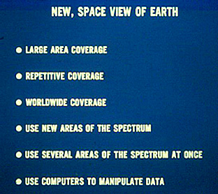
Remote sensing began on the ground,
then moved into the air in the second half of the 19th Century, next on to
airplanes in the first part of the 20th Century and by the 1960s entered space
as cameras and electronic sensors were mounted on spacecraft to open the era of
satellite remote sensing. Various sensors can process radiation not only in the
visible but in shorter or longer wavelengths within the electromagnetic spectrum
(see below). This chart summarizes the main benefits of satellite remote
sensing:
Now consider this very important
precept or thesis spelled out in bold red letters to accentuate the importance
of remote sensing: Most remote sensing systems (built around
cameras, scanners, radiometers, Charge Coupled Device (CCD)-based detectors,
radar, etc.) of various kinds are the most widely used tools
(instruments) for acquiring information about Earth, the planets, the stars,
and ultimately the whole Cosmos. These normally look at their targets from a
distance. One can argue that geophysical instruments operating on the Earth's
surface or in boreholes are also remote sensing devices. And the instruments on
the Moon's and Mars' surfaces likewise fall broadly into this category. In other
words, remote sensing lies at the heart of the majority of unmanned (and
as important tasks during some manned) missions flown by NASA and the Russian
space agency, as well as programs by other nations (mainly, Canada, France,
Germany, Italy, India, China, Japan, and Brazil) to explore space, from our
terrestrial surface to the farthest galaxies. NASA and other space agencies
have spent more money (the principal writer [NMS] estimates this sum to
be in excess of $500 billion dollars) on activities that - directly or
indirectly - utilize remote sensors as their primary data-gathering instruments
than on those other systems operating in space (such as Shuttle/MIR/ISS and
communications satellites), in which remote sensing usually plays only a
subordinate role. Add to this the idea that ground-based telescopes, photo
cameras, and our eyes used in everyday life are also remote sensors, then one
can rightly conclude that remote sensing is a dominant component of the
scientific and technical aspects of human activity - a subtle realization since
most of us do not use the term "remote sensing" in our normal
vocabulary.
Having made this "sales pitch" let
us turn the now convinced to a brief look at the history of Remote Sensing
(covered in further detail on page I-7).
This history is intimately tied in some of its aspects to the Space Program,
whose early highlights will be reviewed beginning with the fifth paragraph down.
But first a short synopsis of remote sensing efforts from aerial platforms above
the Earth.
The practice of remote sensing can
be said to have begun with the invention of photography. Close-up photography
(Promimal Remote Sensing) began in 1839 with the primitive but amazing images by
by the Frenchmen Daguerre and Neipce. Distal Remote Sensing from above ground
began in the 1860s as balloonists took pictures of the Earth's surface using the
newly invented photo-camera. Most photos were made from tethered balloons but
later free-flying balloons provided the platform. The earliest balloon photo was
made of Paris in 1858 by Honore Daumier but this historic first has been lost.
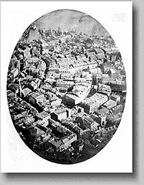
The photo below from a balloon anchored in Boston, made in 1860, is the first
aerial photo surviving in the U.S. Balloons were used for reconnaissance during
the Civil War; legend has it that General McClelland had a battlefield photo
made from such an aerial post but it has disappeared.
NOTE: Each image throughout this Tutorial will
have a caption that is accessed simply by placing your mouse on the lower right
portion of the image.
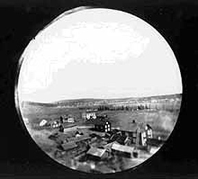
It is a little known fact that the
first aerial photo taken from a rocket was made by the Swede Alfred Nobel (of
Nobel Prize fame) in 1897. Here is the picture he obtained of the Swedish
landscape:
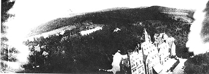
 Perhaps the most novel platform
at the beginning of the 20th century was the famed Bavarian pigeon fleet that
operated in Europe. Pigeons at the ready are shown here, with a famed 1903
picture taken of a Bavarian castle beneath (the irregular objects on either side
are the flapping wings.
Perhaps the most novel platform
at the beginning of the 20th century was the famed Bavarian pigeon fleet that
operated in Europe. Pigeons at the ready are shown here, with a famed 1903
picture taken of a Bavarian castle beneath (the irregular objects on either side
are the flapping wings.
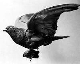
O-3: What is an obvious disadvantage in using this primitive pigeon system? ANSWER
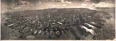
In 1906 interest in getting a panoramic view of the destruction in San Francisco, California right after the catastrophic earthquake prompted an ingenious effort by "flying" cameras on kites. Here is the resulting composite photo of part of the city along and in from the wharves in San Francisco Bay.:
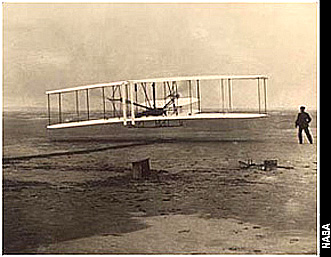
Ever since the legend of Icarus in ancient Greek mythology, humans have been possessed by the urge to emulate the birds and fly themselves. One can point to the famed flight of Wilbur and Orville Wright on 1904 as the first real triumph of making us airborne through use of combustible fuel - in a sense this can be singled out as the first tiny step into Space.
Aerial photography became a
valuable reconnaissance tool during the First World War and came fully into its
own during the Second World War. Both balloons and aircraft served as platforms.
The possibility of conducting
"aerial" photography from space hinges on the ability to use rockets to launch
the equipment, either up some distance to then fall back to Earth or into Earth
orbit. Page 7 in the Introduction describes the earliest successes. Rocketry can
be traced back to ancient times when the Chinese used solid materials, similar
to their firecracker powders, to provide the thrust. In the 19th Century, the
famed French science fiction writer, Jules Verne, conceived of launching a
manned projectile to the Moon (in his book "From the Earth to the Moon", which
formed the inspiration for this writer's [NMS] first presented science paper on
rocketry to his high school Science Club). In the first half of the 20th
Century, a leader in rocketry was Robert Goddard (1889-1945) after whom Goddard
Space Flight Center (where this Tutorial is based) was named. Below is a 1926
photo of Dr. Goddard with one of his first liquid fuel rockets (the motor is on
the top of this 10 foot vehicle [it would break free from the frame holding it
up]).
The logical entry of remote sensors
into space on a routine basis began with automated photo-camera systems mounted
on captured German V-2 rockets, launched out of White Sands, NM. These rockets
also carried geophysical instruments in their nose cones, which were returned to
Earth by parachute. (The writer [NMS] during his Army service at Fort Bliss, El
Paso, TX in 1946-47 was doubly privileged. First he was part of a group of GIs
assigned to search for a missing instrument package in its nose cone. Then, in
Spring 1947, as a Post newspaper reporter, he interviewed Dr. Wernher von Braun
- the guru of post WWII rocketry - and was present during a V-2 launch. Little
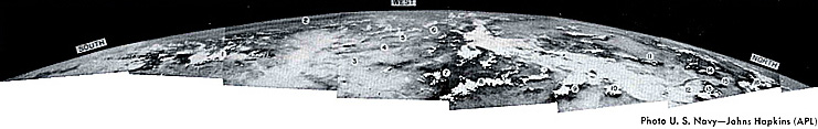
did I realize then that Space would become my career.) Below is an example of
one of the first photo pictures returned from a V-2 firing, along with a list of
specific localities recognizable in this view covering 800000 square miles of
the western U.S. and showing the Earth's curvature:
The modern Space program is held by
many historians to truly have begun with the launch of Sputnik I by the Soviets
on October 4, 1957 (like many noted events that stick in one's memory, the
writer recalls vividly exactly where he was as the news was read over a radio
while he was eating breakfast in a cafeteria in Casper, Wyoming at the start of
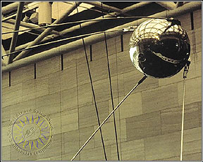
a day of geological field work). Here is a full scale model of the first Sputnik
(about the size of a basketball, weighing 83 kg [182 lb]), with radio and one
scientific instrument), on display at the National Air and Space Museum in
Washington, D.C.:
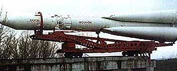
This tiny satellite was hurled into space by the Semiorka rocket, seen below.
The Soviet program was led by Sergei Korolev. An interesting perspective on the
world-stunning effects of this pioneering launch can be read at this Web site.
Several larger Sputniks soon
followed, each with scientific payloads. The U.S. launched its first orbiting
satellite, Explorer 1 in January, 1958, followed shortly by the Vanguard series
(see page
Intro-1a) for more details. Much more about the history of Man in Space is
reviewed in Appendix 1. But this is a good moment to honor
three of the "Titans" of the U.S. space program. In the picture below Wehrner
von Braun is on the right, James Van Allen (Univ. of Iowa), is in center, and
William Pickering, first Director of the Jet Propulsion Laboratory (who died
March 16, 2004 at the age of 93) is on the left; they are holding a life size
model of Explorer 1 which Van Allen developed to explore the particles and
radiation around the Earth (and in so doing, discovered the radiation belts that
bear his name):
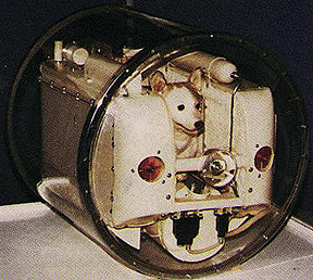
Thus began the Space Race. While
the bulk of launches since 1957 have been unmanned saellites, the real prize
from the prestige viewpoint was putting living creatures into orbit in space.
The Soviets won that effort by orbiting the dog Laika but without returning him
to Earth. This Russian "stray" was trained beforehand and survived for several
hours once in orbit, only to die from overheating.
With trepidations owing to the loss
of Laika, the Soviet program stilled opted to put a man (a cosmonaut) into
orbit. That achievement was garnered by Yuri Gagarin in April 12, 1961. Here he
is with comrades as he prepared to enter Vostok I:
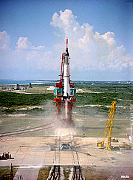
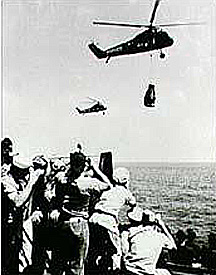
The U.S. space program, now behind
in the manned race, succeeded in placing Alan Shepard into suborbital flight (15
minute duration) on May 5, 1961. He rode a small capsule named Freedom, part of
the Mercury series of flights. Below is a Mercury launch and a photo of
Shepard's capsule after it reached the Atlantic Ocean and was retrieved by
helicopter:
John Glenn, an intrepid U.S. Marine
Corps pilot, won the honor of being the first American (astronaut) to fully
orbit Earth on February 20, 1962.
Glenn later gained fame as a U.S.
Senator and as the first senior astronaut to return to space, 36 years later, on
the Space Shuttle (STS-95) on October 29, 1998. Up to this point we have talked in
general historical terms about what is often termed "space flight", and we will
elaborate further on the topic on this and the next page, and obviously
throughout the Tutorial. But, some of you may decide to get further insight into
the mechanics and history of operating men and machines in space. Now may be an
appropriate time, by reading through The Basics of
Space Flight as prepared by staff of the NASA/Cal Tech's Jet Propulsion
Laboratory (JPL) and clicking on Table of Contents, then reading all or
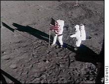
selectively choose what is of personal interest. America's space race sprung into
high gear with the dramatic speech by President John F. Kennedy on May 25, 1961
commiting the U.S. to land on the Moon before the end of that decade. The
American Space Program sprinted rapidly to world leadership because of that
challenging goal, which was met with the landing of the Eagle module on the
lunar surface in July 20 of 1969.
But, after this invaluable
historical diversion, let us return to our consideration of how remote sensing
contributed to the overalll exploration of Earth, the planets, and the Universe
beyond. After the launch of Sputnik in 1957, putting film cameras on orbiting
spacecraft became possible. The first cosmonauts and astronauts used hand-held
cameras to document selected regions and targets of opportunity as they orbited
the globe. Sensors tuned to obtain black and white TV-like images of Earth flew
on meteorological satellites in the 1960s. Other sensors on those satellites
made soundings or measurements of atmospheric properties at various heights. The
'60s also record the orbiting of the first communications satellites.
O-4: On TV, you are most likely to
encounter a satellite remote sensing product of what kind (hint: think local
news)? ANSWER
As an operational system for
collecting information about Earth on a repetitive schedule, remote sensing
matured in the 1970s, when instruments flew on Skylab (and later, the Space
Shuttle) and on Landsat (early on, called ERTS), the first satellite dedicated
to mapping natural and cultural resources on land and ocean surfaces. A radar
imaging system was the main sensor on Seasat, launched in June, 1978. In the
1980s, a variety of specialized sensors - Coastal Zone Color Scanner (CZCS),
Heat Capacity Mapping Mission (HCMM), and Advanced Very High Resolution
Radiometer (AVHRR) among others - orbited primarily as research or feasibility
programs. The first non-military radar system was JPL's Shuttle Imaging Radar
(SIR-A) on the Space Shuttle in 1982. Other nations soon followed with remote
sensors that provided similar or distinctly different capabilities. By the
1980s, Landsat had been privatized and a widespread commercial use of remote
sensing had taken root in the U.S., France, Russia, Japan and other nations.
Much of this growth was, and is still being, driven by the increasing awareness
that Earth's environments are in peril from man's activities and misuses.
O-5: Where might you have seen a
Landsat image before? ANSWER
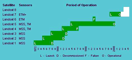
It is generally agreed that Landsat
set the stage for the advent of these other satellite systems in that it
demonstrated the power and versatility of multispectral imagery for observing
the Earth for purposes of monitoring its natural and manmade features over time,
from which the many applications of remote sensing have now become important in
managing our planet's "health" and the utilization of its resources. Since 1972,
six Landsats have been orbited successfully (Landsat-8 did not fly on this
schedule; plans to send it into orbit are still being evaluated). Here is the
history of this highly successful program:
So, how is remote sensing actually
done from such satellites as Landsat, or for that matter, from airplanes
or on the ground? Remote sensing uses instruments that house sensors to view the
spectral and spatial relations of observable objects and materials at a
distance, typically from above them, or in astronomy, by looking out. Geophysics
(mainly gravity, magnetic, and seismic surveys; also external fields) is
considered by many to be a form of remote sensing. But, except for three pages
in the Introduction that summarize doing geophysics measurements from space, we
will confine our study in this Tutorial mainly to methods and applications of
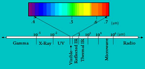
spaceborne sensors that produce images and thematic maps. Most methods are based
on sensing of photons (quantum particles that have a wide range of energies; a
specific photon will have some energy value that has its own unique
corresponding frequency [number of cycles of a sine waveform per unit time]) in
the electromagnetic (EM) spectrum.. Here is a simple EM Spectrum Chart,
with different wavelength intervals named according to common usage in remote
sensing (the wavelength units are in micrometers (µm); a micrometer is
1/1,000,000 of a meter.
This term EM Spectrum refers
to the distribution of radiant energy as a function of wavelengths (distance in
metric units between successive wave crests in an oscillating sine wave, which
for radiation is the trace of a forward moving photon as it revolves 360°
through one cycle) or their inverse, frequencies (number of cycles per second)
presented usually as a chart or diagram with highest frequencies (shortest
wavelengths) at one end and lowest frequencies (longest wavelengths) at the
other. Radiation may be continuous (no break in the range of wavelengths), its
plot consisting of a sequence of all wavelengths over a spectral range whose low
and frequencies are at some beginning and end values. It can also be discrete,
i.e., photon energies are associated with specific, generally narrow wavelength
intervals, with radiation outside these intervals being absent (these
discontinuous intervals are representative of energies released when atomic or
molecular species are excited in specific ways [determined by quantum physics]).
Thus, chemical elements, when excited by thermal or electrical energy, give off
EM radiation at discrete (particular) wavelength values unique to each element
species; these may appear as lines in a spectrogram made by dispersing the
radiation using a prism or diffraction grating..
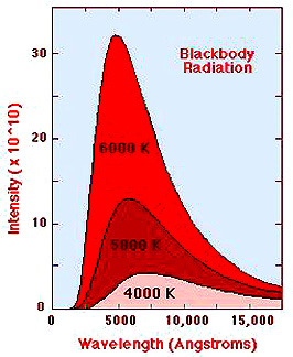
One type of a continuous spectrum
is the blackbody radiation (BBR) emitted by all bodies whose temperature is
above absolute zero. A given BBR spectral plot, characterized by a total
spectral interval fixed on end points of specific wavelengths, is determined by
the thermal state of the object sensed and varies in "area under the curve" (the
plot) and peak intensity, both determined by the surface temperature of the
body. BBR curves for three stars of differing surface temperatures illustrate
this type of radiation; note that as temperatures increase the radiation
intensity also increases and the peak wavelength decreases.
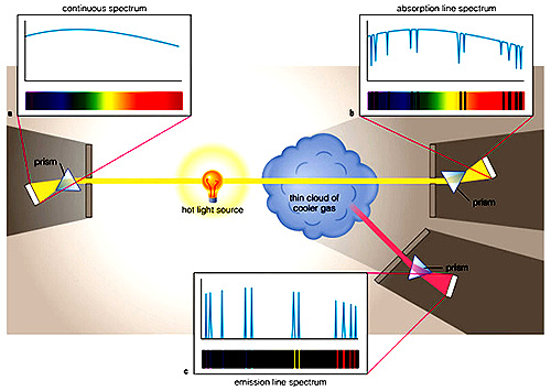
To synposize these last ideas about
electromagnetic radiation, consider this diagram:
Photons are emitted from a hot
source (the Sun, an electric light, etc). The spectral curve for this condition
or mode is like the above BBR curves. Now this light passes through a target, in
this instance a cloud containing atoms and molecules. On the right is an
absorption spectrum in which the black lines are at wavelengths characteristic
of elements or molecules that absorb some of the photons of specific energies
(proxied by their characteristic wavelengths). At the same time, some of these
photons cause atoms and molecules in the cloud to be excited such that they give
off (emit) radiation at particular wavelengths, as shown in the bottom
spectrum. In actual practice in remote
sensing, classes of features (leaves, soil, rock, buildings, etc), upon
excitation reflect or emit radiation that produces plots of photon energy
variations as a function of wavelength or frequency that comprise characteristic
spectral signatures (curves) (see below). The ideas in this paragraph are
treated in detail in the Introduction that follows this Overview. Most remote sensing data consists
of receiving and measuring reflected and/or emitted radiation from different
parts of the electromagnetic spectrum. Those parts of the spectrum most commonly
sampled are the ultraviolet, visible, reflected infrared, thermal infrared,
and microwave segments. Multispectral (or the closely related
multiband data consist of radiation collected over sets of
electromagnetic radiation that individually extend over (usually narrow)
intervals of continuous wavelengths within some part of the spectrum. Each
interval makes up a band or channel identified by a color (if in
the visible), a descriptive label (e.g., Near IR), or a specified range of
wavelengths. The data are utilized by computer-based processing to produce
images of scenes (Earth's surface and atmosphere; planets; cosmological
features) or to serve as digital inputs to analytical programs (see Section 1
for a thorough examination of imaging techniques and categories of
analysis). Multiband images collected by one
sensor will usually show notable differences from one band to the next. This is
because the radiation from point to point in an array of sampling areas making
up a scene will vary depending on the reflectance or emittance response of the
various features/materials are different within an interval, and different again
when other bands are examined. The band to band response (in terms of magnitude
or intensity of radiation) of any such point can be connected to become the
spectral signature for a given feature or class of materials. Different
features/classes have differing and normally distinctive signatures. Much of the ideas given in the
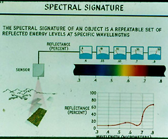
preceding three paragraphs can be summarized in this diagram:
In this case, the target is a field
of actively growing crops - the main components are thus vegetation, soil, and
moisture. The detailed spectral signature for this composite of materials is
shown in the lower right. Some fraction of the incoming solar radiation is
reflected towards a sensor above (on an aircraft or spacecraft). While it is now
possible for a sensor system to almost duplicate the signature using the mode
called hyperspectral remote sensing, in this example the broadband mode,
initially the normal configuration for obtaining reflectance measurements and
still in common use, is illustrated here. Thus the sensor employs bandpass
filters to break the reflected radiation into discrete intervals (bands)of
continuous wavelengths, each consisting of a segment of the EM spectrum (red,
green, infrared, etc.). The radiation consists of photons that impign upon a
plate that converts the photon energy to a voltage (photoelectric effect). At
the instant of sampling this radiation, each band will have some voltage value
(indicated on the dials). Assuming proper calibration of each band (channel),
this voltage is a measure of the reflectance from the target composited for each
spectral interval. The resulting values represent a crude approximation of the
spectral signature. However, even these few values may be sufficiently distinct
to establish the identity of the target. Obviously, the more bands (and narrower
bandwidths), the better is the discrimination. To whet your appetite for remote
sensing and to familiarize you with some of the principal types of image
products that are used to monitor and document the Earth's surface, we will now
present an example of multispectral images and then a sequence of space images
of an area of the United States that occupied centerstage during February of
2002:
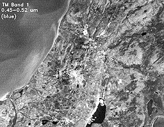
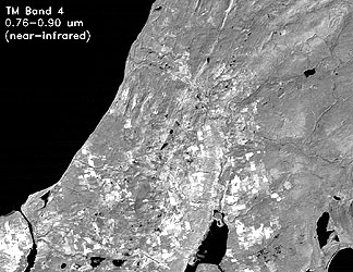
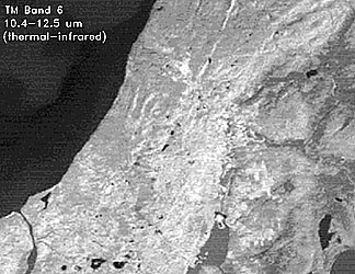
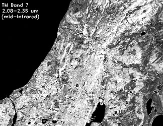
We will illustrate these ideas by
showing images representing 4 of the 7 bands acquired by the Thematic Mapper
(TM), the main sensor on Landsats 4 through 7. Each image was constructed from
numerical values called Digital Numbers (DNs) which correlate with the intensity
of reflected or emitted radiation averaged for the spectral interval (Band)
displayed; the DNs in this case range from 0 to 255 in whole number increments.
Levels of gray in the resulting image range from black (DN = 0) to white (DN =
255) with shades of dark gray to very light gray associated with increasing DN
values. The scene, a subset of a full Landsat TM image, shows the western shore
of the Keweenaw Peninsula of northern Michigan (for this and other related
images, link onto the Michigan
Technological University Web site). Wavelength intervals (in micrometers)
are shown; check the captions (cursor on lower right) for more information.
For bands 1, 4, and 7, the darker
(gray scale) tones in these black and white renditions represent low (intensity)
reflectances whereas light tones are high reflectances. In band 6 what is
measured is emitted radiation which becomes more intense (leading to lighter to
white tones) with higher temperatures. Starting with Band 1, pick out certain
features (a pattern of usually uniform gray tones), without concern about their
identities, and find the gray tones at equivalent points in the other three
images - this will give you a feel for how reflectances (or emittances in Band
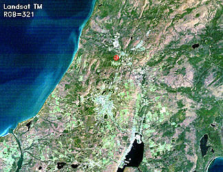
6) vary as a function of wavelengths used to monitor features/classes. Combinations of any 3 of the 7
bands on TM can be registered spatially and then each assigned to one of the
three primary colors: blue, green, red to yield what is called a color
composite. This can be done photographically using color filters or in a
computer display in which the colors are determined by the assignment (using an
image processing program) of a given band to one of three color guns in the
monitor (and the remaining two bands each to the remaining colors). For the TM,
the most frequently used combination is Band 2 = blue; Band 3 = Green; Band 4 =
red, giving the standard false color version in which most of the reds and
off-reds are the color signatures of vegetation. This is present here as a
larger subset showing nearly all of the Keweenaw Peninsula:
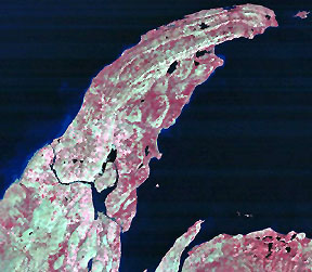
Below is another combination
applied to the smaller using 3-red, 2-green, and 1-blue. In this image, for the
"fun of it" locate where this subset is in the image above and try to identify
(give them names, like water, town) features you recognize.
This brief primer on the appearance
of individual multispectral bands and on making color composites from
combinations of three bands (or other variables) from one (or perhaps two or
more) sensors designed to scan the target (Earth's surface; a galaxy, etc.) as
an array of spatially distinct points (in many cases, the sampled point can be
called a pixel (picture element) should help you to
appreciate some of the images from various sensors and sources to follow in this
Overview. Again, more details on this subject are given in the Introduction and
in Section 1. The MSS was the key sensor of
Landsats 1, 2, and 3 and was also on 4 and 5 to retain continuity of image types
for those doing multitemporal studies. However, on 1-3 there was a second
sensor, almost forgotten today since it did not prove to have the versatility of
the MSS. This was the RBV, or Return Beam Vidicon, a television camera that
produced images much like early home television systems. One Landsat 1, there
were three bands, two in the visible (red and green) and one in the
near-Infrared. The resolution was, like the MSS, 80 meters. The RBV was seldom
used on Landsat 2. The RBV on Landsat 3 was panchromatic (single image covering
0.5 to 0.75 µm), imaged in four quadrants, and had 30 meter resolution. This
allowed merger of MSS and RBV images to give an effective higher (30 m)
resolution. The "hallmark" of an RBV image is a series of small crosses ("+")
called reseau marks regularly spaced as an aid in geometric (spatial)
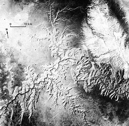
corrections. RBV pictures are hard to find on the Internet or textbooks. Here is
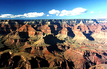
one example showing the Grand Canyon, imaged by the first RBV: From space the extent and width of
the Grand Canyon is made obvious. But space imagery cannot capture the grandeur
of this geologic wonder, as is evidenced in this ground photo.
The Internet is a prime source for
information on almost every aspect of remote sensing. Many sites offer good
overviews of satellite remote sensing. For a general listing of these sites,
consult Remote
Sensing Tutorials and Training Courses. One that has recently appeared, and
provides an excellent synopsis of the main principles and applications, has been
constructed by the Canadian Center for Remote Sensing. Click here
if you want to view it now, or at your leisure. Another of merit is the Remote Sensing Core
Curriculum, project which highlights a new educational approach now under
development. A thorough treatment of the basics of remote sensing, prepared by
the Japanese Association of Remote Sensing, is online at this mirror
site. A somewhat briefer review has been prepared by Harrison and
Jupp. A recent NASA-supported initiative in curriculum development is
described at the Geospatial
Information Technology website of the University of Mississippi. For a broad
perspective on how remote sensing has flourished in the last 30 years, one needs
only to check out the still growing number of U.S. and International
organizations - government, university, and private - that are largely concerned
with various facets of remote sensing. A listing of most of these is found at The
Remote Sensing Organizations site. Another source of information on various
remote sensing tutorials and related topics is located as a link on the Home
Page of the Remote Sensing Tutorial; for those accessing the RST through the CD,
we provide this link here as the Carstad site.
Lastly, for those who might wish to build or expand their knowledge and
background in several sciences that are relevant to remote sensing, we strongly
recommend exploring the PSIGate site maintained by
the University of Manchester (England) that has many useful links in Astronomy,
Earth Science, and Physics. Having surveyed some basic
principles and examples of remote sensing and its products, we now move on to
the aforementioned sequence of various types of imagery that relate to a major
event in Utah during February, 2002. We turn to The Salt Lake City, Utah region,
site of the 2002 Winter Olympics. This should help you appreciate the
advantages of both multiplatform, multisensor, and multitemporal data and
imagery.
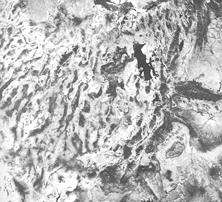
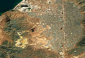
To set the Salt Lake City area into
a large, i.e., regional context, look first at this Daytime Thermal image made
by the Heat Capacity Mapping Mission (HCMM):
The Great Salt Lake is the dark,
elongate feature in the upper right quadrant. It is dark because, thermally, it
is cool and in conventional thermal images cold features tend to be dark gray to
black and warm in light gray to white. The mountain chains show up moderately
dark because they are cooler - at higher altitudes - than lowlands and basins.
Next to the Great Salt Lake just to its lower right is Salt lake City. The dark
vertical area to SLC's right is the Wasatch Range - home of many Olympic events.
The east-west chain of mountains to its east is the Uinta Mountains. Many
elongate dark features, running mostly up-down in the image, are individual
mountains that make up the Basin and Range tectonic and geomorphic
provinces.
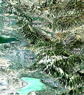
To put the "venue" of this great
sports event into context with its surroundings, at a regional scale, we'll
start with one of the typical aerial oblique photos taken by the astronauts on a
Space shuttle mission; read the caption (click on picture) for a general
description.
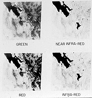
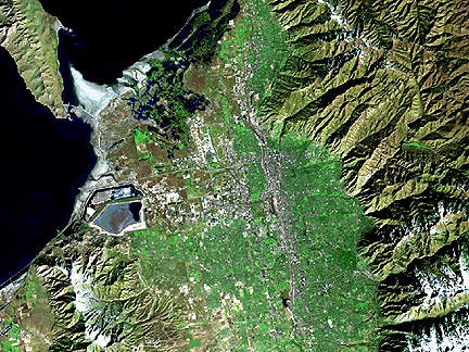
Now, we introduce you to a
characteristic unmanned satellite image: Shown first are the four individual
band images made by the Landsat 1 Multispectral Scanner (MSS; 79 m resolution)
presenting a view of north-central Utah taken just 15 days after launch of
ERTS-1 (the name given this satellite before it and its successors were renamed
the Landsat series), on August 7, 1972. The bands are identified in the caption
(note: these are somewhat degraded in quality because they were scanned from a
35 mm slide; the two IR band images are also not well-balanced in gray tones
owing to rather poor tonal stretching as those in the image-processing lab were
still learning how to generate good quality photo prints).
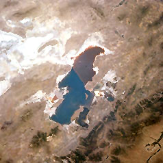
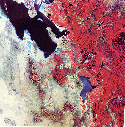
The scene below is a an early
(Summer of 1972) Landsat (ERTS-1) false color image (185 km [110 miles] on a
side) that helped to generate widespread interest in using satellites to monitor
the Earth's surface. Images of this type are made by sensors that receive
reflective light which is split into several Bands (made by subdividing both the
visible and the near infrared spectrum into narrower wavelength intervals), each
with different tonal intensities (gray levels) in its image. Three of the band
images are then recombined (registered) photographically (or by a computer
program) using red, green, and blue filters (this idea, treated very briefly
here but in detail in the Introduction. The combination of bands and filters can
vary, giving rise to color composites that differ in colors associated with
different features depending on the band/filter pairing.
The version shown here is a
composite made by projecting the MSS Band 4 (green wavelength interval) through
a blue filter, 5 through green, and 7 (IR) through red. The right side of the
image is bright red, which is the normal color for thick forests and grasslands
as rendered in a standard false color image in which we associate red with
healthy vegetation that is usually very bright (high reflectance, appearing in
light tones) in the near-infrared (see page I-13
in the Introduction Section for the explanation of color response and
assignment). This widespread red area coincides with the high Wasatch Mountains
that run east of the block-fault mountains and deserts (gray-tan tones) of
western Utah. Other reds in small patches mark the farmlands of the desert
plains whose potential inspired Brigham Young to settle his group in this
"promised land". The Great Salt Lake occupies part of the upper scene. Lake Utah
(bluer because of silt) is to its south. We challenge you to find the
metropolitan area of Salt Lake City in this image. O-6: This is a good moment to begin
to associate locations and features within a space image such as Landsat with
their counterparts on a map. Using a U.S. Atlas or a state map, fit the Landsat
image to its equivalent map area. In addition to places mentioned above, also
find these features: The small cities of Ogden, Orem, and Provo; Park City; Utah
Lake; the Bingham Open Pit Copper mine in the Oquirhh Mountains; large areas
devoted to agriculture; heavily forested lands; desert flats. Also, in your
atlas, if it is nearly new, the shape of the Great Salt Lake may differ from
that in the image; why? Finally, why is the central part of Salt Lake City
(which appears as a long darker blue strip) so narrow, when the greater area of
the city and suburbs seems to appear reddish? ANSWER
Below this image, we place a
subscene (part of the total area covered; the image was made using a subset of
data points sampled by the MSS) image of the same area made from a Landsat-7
image acquired in the late 1990s. Landsat-7 had a different version of the
Thematic Mapper called the ETM+ (or Enhanced Thematic Mapper) which included a
separate 15-meter resolution panchromatic mapper and improved the thermal band
resolution from 120 to 60 meters. For the moment, just look it over and try to
note any conspicuous differences between it and the corresponding area in the
Landsat-1 image. We will take this comparison up again a few paragraphs
later.
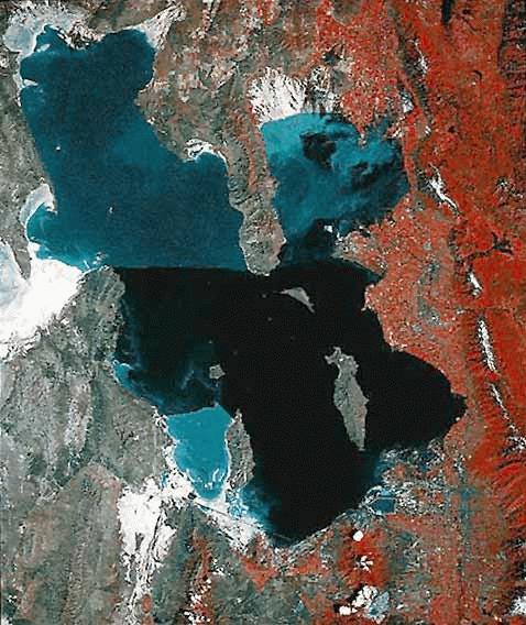
If you look intently at the
Landsat-1 image, you may see a slight tonal difference along a straight, sharp
boundary; this is due to a cutoff of water circulation by the Union Pacific
railroad causeway. This is much easier to see in this next near-true color image
made by the MODIS sensor onboard Terra (see Section 16). The tonal discontinuity
is almost "invisible" in the Landsat-1 image because the multispectral sensor
(MSS) onboard does not have a blue band that would have picked out the presence
of silt (which increases the reflectivity of the water, producing a ligher tone
in the blue region of the visible spectrum) in the Upper Great Salt Lake.
Notice in the Landsat-7 image shown
above that this straight border is now altered to a bend in which the two
segments appear to meet at a high angle. The left (western) segment is still a
straight line but the right (eastern) segment has a blurred boundary. The area
to its north was mostly saline silt deposits in the 1972 image but water has
since spilled into the land above the train causeway. Close to the tracks, the
water to the north is relatively clear but the blue silt tones start to show up
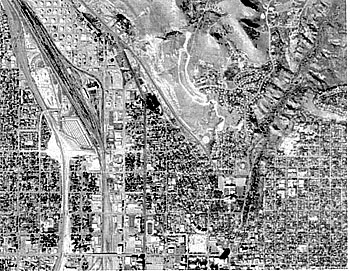
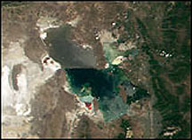
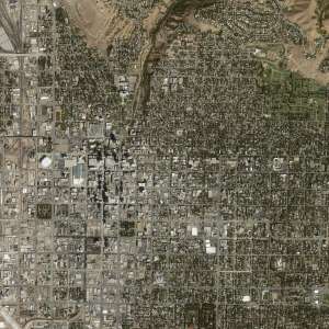
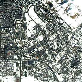
a short distance further up. In case you had difficulty in
pinpointing the city, this next view should help. It is a Landsat-5 Thematic
Mapper (TM; 30 m resolution) natural color image of the immediate urban
area. It also demonstrates the improvement in detail that has transpired in the
later Landsats owing to this new sensor.
These images, of course, are
vertical (straight down) views. To acquaint you with looking at Earth this way,
we draw upon a more familiar viewing vantage by showing this near-horizontal
aerial view of the city and the Wasatch Front to its east. (The famed Mormon
Tabernacle is the multi-spired building near the center). 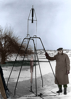
![]()


 Note: to convert Angstroms to the more common micrometer unit
(µm), multiply by 10-4, or 1/10000
Note: to convert Angstroms to the more common micrometer unit
(µm), multiply by 10-4, or 1/10000
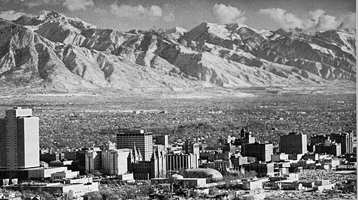
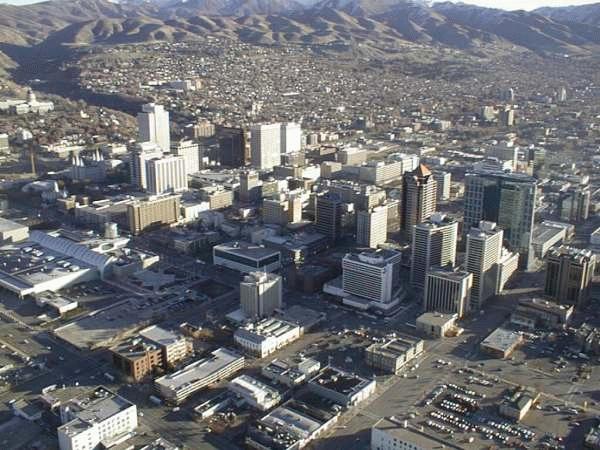
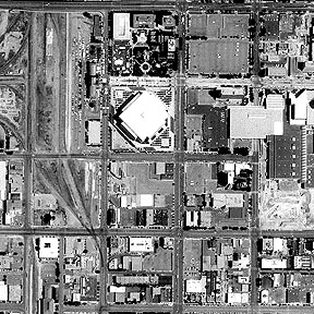
Compare the downtown area shown above in a photo taken in the mid-1960s with a photo taken in 2001. Try to determine which major buildings (some are high-rise) have been added to the skyline since the '60s.
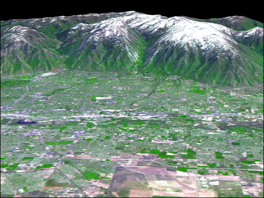
As will be repeatedly demonstrated throughout the Tutorial, space imagery can be combined digitally through specialized computer processing which uses a digital elevation data set to produce what is known as a perspective view (as though you were approaching the scene in a low flying aircraft and looked ahead; much like the above aerial photo). Here is a Landsat-5 perspective of the Wasatch Front with much of Salt Lake City in the foreground.
Another Landsat perspective view from a different direction shows the location of the principal Olympics venue sites both in Salt Lake City and the mountains to its east:
The Wasatch Mountains show up as even more imposing in this perspective view of Salt Lake City made from Shuttle Radar Topography Mission (SRTM) data, in which the vertical elevations have been exaggerated (often the custom when relief [difference in elevation] warrants emphasis):

To get a more intimate feel for the downtown part of Salt Lake City, here is two high resolution images made by the IKONOS satellite (see next page). The first, in color, shows much of the downtown (at 4 m resolution), including part of the University of Utah. The second depicts, at 1 m resolution how city blocks in this town tend to be square; the two large buildings in it can be located near the left center edge of the first image.
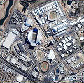
We can zero in on the Olympics infrastructure that has been home to more than 2500 international athletes. Again, two high resolution IKONOS color images, one taken in the summer of 2001 and below it part of the same area taken during the Winter Games in February, 2002.
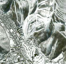
The part of the Olympics that includes downslope sking lies in the Wasatch Range near Park City, just east of Salt Lake City. Here is an IKONOS view which shows the ski trails, and housing to the west:
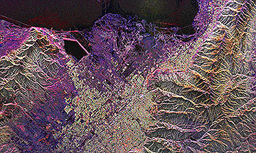
Leaning on your new found familiarity with Salt Lake City, try to find some of the features shown in the above images in this very different-appearing image. This scene was obtained during the SIR-C radar mission carried out by astronauts in 1994. Each of the three radar bands (C, L, X) were assigned color used to generate this "false color" composite (see page 8-7 ). The image is oriented with the top boundary running NE-SW; the Great Salt Lake is the black area below the top.
So far in our excursion in and around Salt Lake City, we have treated you to what might be called "pretty pictures". But, now is a good time to stress the practical use or applications of space imagery. One such use comes under the term "change detection" - determining what features or conditions in a scene have been introduced, modified, or expanded over short to long time periods. Scroll upwards now to the two Landsat scenes (full Ls-1 and subset Ls-7). There are at least three major features or categories that are different (changed) in the lower Ls-7 scene representing a time span of 27 years. Do this before advancing to the next four scenes.
Urban population is one change that you would expect of this lengthy time period. The United States has increased its citizens considerably since 1972. The West, in particular, is experiencing a population boom, both from increased childbirth and from the influx of people from the eastern U.S as well as Mexicans who have emigrated from their native country. Salt Lake City shares this trend, as is evident from this pair of Landsat images. To estimate the extent of the growth, look for street patterns in each image - the major clue is the spread of buildings as the suburbs expand away from the mountains.

 ">
">The most noticeable area of growth occurs in the middle of these images (the 2001 image shows urban/suburban sections of the city in a grayish tone; this is probably due to that image being taken at a different time of the year). Note the large, irregular "scar" in light brown in the lower left quadrant of each image. This is the Bingham Canyon copper mine, located in the Oquirhh Mountains. This is the largest open pit mine in the world (note the increase in peripheral size in the 2001 image). You will see this mine again in an enlarged image subset at the bottom of Page 5-4.
The second pair of Change Detection images focuses on the southern end of the Great Salt Lake. Significant differences between the 1972 and 2001 Landsat images occur at several places, In the 1972 scene, the peninsula of land near the bottom center is tied to the shore with all land exposed. By 2001, that peninsula has been cut off from the mainland. This is the result
We return for the moment to what has happened in and around the Great Salt Lake since 1972. Two Landsat images, the top taken in 1972 and the bottom in 2001, will allow easy comparison that facilitates picking out the changes in 29 years.

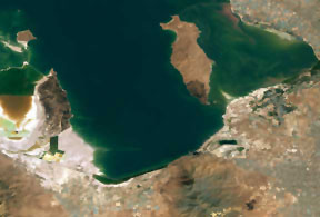
The most obvious modification noted
in the 2001 image is that the peninsula at the southern end of the Lake has
become isolated (into Antelope Island) owing to the lake surface level's rise
since 1972. At first, this seems counterintuitive since the ultimate fate of
lakes is for them to dry up (some as rapidly as a few thousand to 20000 years).
But this is not a uni-directional process. Changes in climate from dry to wet
and reverse can have measurable effects over spans of decades. In 1963, the
Great Salt lake had shrunk from the hundred year average of 4200 square miles to
a value of ~950 square miles. This shrinkage was the consequence of a continuing
drought that began in the 1950s. By 1972, the area covered by the lake had
extended to about 2500 miles2. At that time there was still a land
bridge to Antelope Island. By 2001, that bridge was inundated, restoring the
peninsula to island status. Elsewhere in the subscenes being compared, a tongue
of sandy land on the southeast corner of the lake was resubmerged by (actually
before) 2001 and the lowlands adjacent to a mountain outlier in the southwest
corner have become partially covered with shallow water that supports
vegetation.
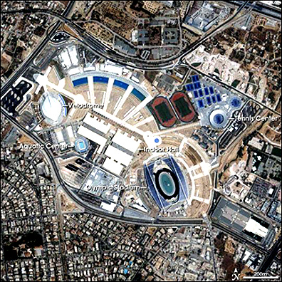
The Summer Olympics of 2004
are being held at the end of August in the country where a "miniature" scale
Olympics was first put on almost 2400 years ago: Greece. The 2004 Olympics will
be held in and around Athens, at six venues shown in this SPOT-5 image. Below it
is an IKONOS small area (but high resolution) image of the main facilities at
the Sports Complex (1).
Now, let's leave the specificity of
a single scene (both large and small areas of coverage), used to introduce you
to some of the ways in which satellite imagery can depict the Earth's surface,
and return to the more general overview of what Remote sensing is all about and
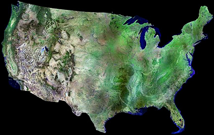
can do in practical ways. In addition to regional and local scale coverage,
sensing from satellites allows images to be created that can envisage the full
Earth or entire continents, relying either on single looks from geostationary
satellites or mosaics constructed from numerous individual scenes.. Here, for
example, is the quasi-natural color view of the 48 continental U.S landmass
(Courtesy Earthsat Corp, Rockville, MD) made from summer AVHRR (see page 14-2)
imagery. Notice the regionally variable distribution of vegetative cover
(green). (Examples of mosaics are found in Section 7 and elsewhere.)
Coming back to one major theme in
this Overview, the purpose, scope, organization and content of this Tutorial: It
will draw extensively on the Landsat satellites for the images of the Earth's
surface you will see, in part because there are so many outstanding scenes
acquired since 1972 but also in part because the writer (NMS) spent most of his
career at NASA Goddard working on data from these satellites. The RST also
utilizes imagery from a variety of sensors operating from land and sea
satellites launched by U.S. government and private U.S. industry and by
governments and commercial firms in other countries. Most of these observe in
the visible, near infrared and thermal infrared spectral intervals, but images
from several radar systems are also included as examples of common space data
sets.
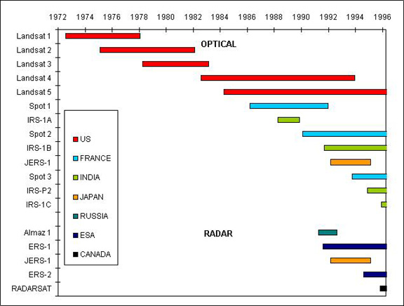
Listed here are the principal
(non-commercial) remote sensing spacecraft flown by the U.S. and other nations
(identified in parentheses) along with the launch date (if more than one in a
series, this date refers to the first one put successfully into orbit. These
fall naturally into three Groups based on their principal applications: Land,
Meteorology, Oceanography. However, many of the satellites provide useful
information for more than one Group: Group 1 - Primarily Land Observers:
Landsat (1-7) (1973); Seasat (1978); HCMM (1978);
RESURS (Russia) (1985); IRS(1A-1D) (India) (1986); ERS
(1-2) (1991); JERS (1-2) (Japan) (1992); Radarsat (Canada) (1995);
ADEOS (Japan) (1996); Terra (1999); Proba/Chris (2001)
------------------ Group 2 - Primarily Meteorological Observers:
TIROS (1-9) (1960); Nimbus (1-7) (1964); ESSA (1-9) (1966);
ATS(g) (1-3) (1966); DMSP series I (1966); the Russian
Kosmos (1968) and Meteor series (1969); ITOS series (1970);
SMS(g) (1975); GOES(g) series (1975); NOAA (1-5) (1976);
DMSP series 2 (1976); GMS (Himawari)(g) series (Japan) (1977);
Meteosat(g) series (Europe) (1978); TIROS-N series (1978);
Bhaskara(g) (India) (1979); NOAA (6-14) (1982); Insat
(1983); ERBS (1984); MOS (Japan) (1987); UARS (1991);
TRMM (U.S./Japan) (1997); Envisat (European Space Agency) (2002); Aqua
(2002)
--------------------
(Note 2: g = geostationary) (Note 3: Nimbus also observed
general land features; e.g., Nimbus 6 carried SCMR, an experimental sensor
designed to obtain information on surface composition) Group 3 - Major use in Oceanography:
Seasat (1978); Nimbus 7 (1978) included the CZCS, the
Coastal Zone Color Scanner that measures chlorophyll concentration in seawater;
Topex-Poseidon (1992); SeaWiFS (1997)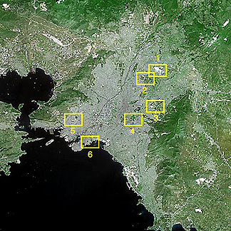
--------------------
(Note 4: NSCAT, the NASA Scatterometer, developed at JPL and launched in 1996 by a Japanese rocket, was designed mainly for oceanographic studies but has provided valuable information applicable to meteorology and land observations.)
Commercial Satellites designed to produce imagery useful to the above Groups started to operate by the mid 1980s. Among the growing number of these privately owned satellites are: SPOT (France) (1986); Resurs-01 series (Russia) (1989; became commercial in the 1990s); Orbview-2 (U.S.)(1997) SPIN-2 (Russia)(1998); IKONOS (U.S) (1999); Quickbird (U.S) (2001); Resource21 (first 4 satellites yet to be launched); EROS A (ImageSat International; Israel) (2000).
A very good review of most of the major satellites dedicated to earth observations and their characteristics, with links (some of which no longer work [404 Not Found]) to parent Web sites, can be called up from these two sites: National Air and Space Museum and University of Wisconsin.
Another site that emphasizes remote sensing and imagery is the Eduspace program sponsored by the European Space Agency (ESA). The site can be accessed by clicking on Eduspace links. Be advised that to get into some of the features at this site, you must be able to register as a member of a teaching institution - primary through college.
Another Website dealing with most aspects of remote sensing is The WWW Virtual Library of Remote Sensing, out of Finland. It has an abundance and variety of links, many of which are worth exploring at some stage in your use of this Tutorial. However, it is not maintained for currency, so that some enticing titles are no longer active.
It helps to picture the dazzling array of operational satellites by looking graphically at launch dates and lifetime of some of those in the above list (primarily land observing satellites) through the year 1996; others since 1997 are listed on a bar chart found on the second page of the Overview.:
This impressive list convinces us that remote sensing has become a major technological and scientific tool for monitoring planetary surfaces and atmospheres. In fact, the budgetary expenditures on observing Earth and other planets, since the the space program began, now exceed $150 billion. Much of this money has been directed towards practical applications, largely focused on environmental and natural resource management. The Table below, put together in 1981 by the writer, summarizes the principal uses in six disciplines.

All of these applications are valid today, and many others have been devised and tested, some of which we introduce in other Sections of this Tutorial. The literature on remote sensing theory, instrumentation, and applications is now vast, including a number of journals and reports of numerous conferences and meetings. The great improvements in computer-based image processing, especially personal computers that handle large amounts of remote sensing data, have made robotic and manned platform observations accessible to universities, resource-responsible agencies, small environmental companies, and even individuals. Geographic Information Systems (GIS) provide an exceptional means for integrating timely remote sensing data with other spatial types of data. The GIS approach (explained in Section 15) stores, integrates, and analyzes information that has a practical value in many fields concerned with decision-making in resource management, environmental control, and site development.
The need for monitoring terrestrial
systems that observe, quantify and map changing land use, search for and protect
natural resources, and track interactions within the biosphere, atmosphere,
hydrosphere, and geosphere has become a paramount concern to managers,
politicians, and the general citizenry in developed and developing nations. This
need has led to a mammoth international program to use a variety of
technologies, centered on observation systems from space, to improve our ability
to oversee and regulate the systems that govern Earth's effective operations.
Among names associated with this concept are the International Geosphere and
Biosphere Programme (IGBP) (a synopsis of which is found at this United Nations
Environomental Program site) and the International Global Change Program
(IGCP). These programs cover a range of research and applications that embrace
primarily climate studies, oceanography, and terrestrial environment monitoring.
National programs include organizations that mainly make ground measurements but
the current availability of suitable satellites flown by several countries leads
to a symbiotic integration of space observations and ground measurements. This
diagram depicts some of the primary topical activities, as described by their
acronyms.
The United States has been the
kingpin in these efforts. Its chief role has been in providing many of the
versatile satellites that make the critical land, sea, and air measurements on a
global scale.
Closely allied to these and other
programs is a new field of the geosciences called Earth System Science.
Many Universities are now offering courses and even majors in this new field of
natural science. When these various programs are
examined closely, as will be done throughout Section 16
of the Tutorial, two principal areas of emphasis underlie the goals and means of
IGBP and ESE: 1) the concept of Global Change, which recognizes that the
Earth's natural systems are constantly modifying, with various diverse aspects
such as atmospheric temperatures, air and water pollutants, and land cover
interacting in often complex ways to alter environments; and 2) Global
Climate, which is often the most important single component of the Earth
System in controlling the changes over time and in different regions of the
Earth. These modifications may be cyclical or unidirectional but generally take
place slowly (almost imperceptibly over short time spans) and thus require
extended, repeated coverage over years to decades using a variety of
observational means (of which satellites are proving the most facile). These two
Logos give URLs (which you must access separately) for these specific U.S.
programs .
These programs will last well into
the first decade of the 21st Century. Starting in 1998, several major platforms
launched with broad complements of sensors supported by continuing operation of
current sensor systems. The programs will have far-reaching impact on all
nations and at least an indirect effect on all people on our planet, as they
address problems and concerns tied to the environment and to resources. When
coupled and integrated with other major data management and decision making
approaches, GIS, ESE, and EOS should evolve into highly efficient implements for
continuous gathering and processing of key elements of knowledge required to
administer the complex interactions between nature and human endeavors.
If you want a preview of how some
scientists apply remote sensing to monitor mankind's influence on the
environment, then go to the Home Page recently added to the Internet by The Consortium for
International Earth Science Information Network. Offline sources of basic
information about remote sensing are the writer's (NMS) still relevant 1982 NASA
Publication RP 1078: The LANDSAT TUTORIAL WORKBOOK; MISSION TO PLANET EARTH:
LANDSAT VIEWS THE WORLD (co-authored with Paul D. Lowman, Jr, Stanley C. Freden,
and William C. Finch, Jr); THE HCMM ANTHOLOGY, NASA SP-465; and (co-authored
with Robert Blair, Jr) GEOMORPHOLOGY FROM SPACE, NASA SP-486.
Here is a list of nine well-known
textbooks that detail most of the fundamentals and applications of Earth Remote
Sensing: An excellent blending of remote
sensing imagery, ground photos, maps, and other types of geographic information
is found in the Atlas of North America: A Space Portrait of a Continent,
published by the National Geographic Society (1986). Also of value are these Periodicals devoted largely to remote sensing methods
and applications: To expand upon the remarks at the
beginning of the Overview, the primary purpose of this Tutorial is to be a
learning resource for college students, as well as for individuals now in the
work force who require indoctrination in the basics of space-centered remote
sensing. In both instances the objective is to offer a background that will
actually be useful in current or eventual job performance to those who may need
to provide input information obtainable from remote sensing into day-to-day
operations. We also think the Tutorial can be an invaluable resource for
pre-college (mostly Secondary School) teachers who want to build a background in
the essential contributions of the space program to society so as to better
teach their students (many of whom should also be capable of working through the
main ideas in the Tutorial). Our hope is that this survey of Satellite Remote
Sensing will attract and inspire a few individuals from the world community who
might consider a specialized career in this field or in the broader fields
allied with Earth System Science (ESS) and the Environment (see below). An
additional goal is to interest and inform the general public about the
principles and achievements of remote sensing, with emphasis on demonstrated
applications. Here is our list of topics chosen
to accomplish these objectives, by providing a comprehensive survey of remote
sensing and its many ramifications. 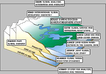
 The program began in the early
1990s under the name Mission to Planet Earth; that program was renamed
Earth Science Enterprise. ESE involves many federal agencies as well as some
private organizations. NASA's role, located primarily at Goddard Space Flight
Center, is to operate the Earth Observing System (EOS) program which will plan,
build, and launch a number of satellites, a list of these being found at this NASA
Headquarters site.
The program began in the early
1990s under the name Mission to Planet Earth; that program was renamed
Earth Science Enterprise. ESE involves many federal agencies as well as some
private organizations. NASA's role, located primarily at Goddard Space Flight
Center, is to operate the Earth Observing System (EOS) program which will plan,
build, and launch a number of satellites, a list of these being found at this NASA
Headquarters site.


Foreword
Overview of this Remote Sensing Tutorial; "Getting Acquainted" Quiz
Introduction to Remote Sensing: Technical and Historical Perspectives; Special Applications such as Geophysical Satellites, Military Surveillance, and Medical Imaging
Section:
1. Image Processing and Interpretation: Morro Bay, California; First Exam
2. Geologic Applications: Stratigraphy; Structure; Landforms
3. Vegetation Applications: Agriculture; Forestry; Ecology
4. Urban and Land Use Applications
5. Mineral and Oil Resource Exploration:
6. Flight Across the United States: Boston to San Francisco; Quiz; World Tour
7. Regional Studies: Use of Mosaics from Landsat
8. Radar and Microwave Remote Sensing
9. The Warm Earth: Thermal Remote Sensing
10. Aerial Photography as Primary and Ancillary Data Sources
11. The Earth's Surface in 3-Dimensions: Stereo Systems and Topographic Mapping
12. The Human Remote Senser in Space: Astronaut Photography
13. Collecting Data at the Surface: Ground Truth; the "Multi" Concept; Hyperspectral Remote Sensing
14. The Water Planet: Meteorological, Oceanographic and Hydrologic Remote Sensing
15. Geographic Information Systems: The GIS Approach to Decision Making
16. Earth Systems Science; Earth Science Enterprise; and the EOS Program
17. Use of Remote Sensing in Basic Science Studies I: Mega-Geomorphology
18. Basic Science Studies II: Impact Cratering
19. Planetary Remote Sensing: The Exploration of Extraterrestrial Bodies
20. Cosmology: Remote Sensing Systems that provide observations on the Content, Origin, and Development of the Universe
21. Remote Sensing into the 21st Century; Outlook for the Future; Final Exam
Appendix A: Modern History of Space
Appendix B: Interactive Image Processing
Appendix C: Principal Components Analysis
Appendix D: Glossary
Unlike a formal course in the subject, with chapters covering principles, techniques and applications in a pedagogic and systematic way, we lead you through a series of Sections focused on one to several relevant themes and topics. Because we can represent most remote sensing data as visuals, we will our organize our instructional treatment around illustrations, such as space images, classifications, maps, and plots, rather than numerical data sets. These data sets are the real knowledge base for application scientists in putting this information to practical use. (Much of this material has been acquired by direct downloading off the Internet. We are grateful to the source organizations and individuals but, for the most part, we do not acknowledge each contribution per se.) Descriptions and discussions accompany these illustrations to aid in interpreting the visual concepts. "Standard" space images, particularly those from Landsat sensors, are usually the focal points of a Section, but we frequently add special computer processed renditions with ground photos that depict features in a scene and descriptive maps where appropriate.
We also call out numerous links to other remote sensing sources and to various continuing or planned programs. Some of these programs are federal or international programs such as ESE, whereas, others are programs from educational or commercial organizations that provide training and services. These links, in turn, have their own sets of links, which, as you explore them, will broaden your acquaintance with the many facets of remote sensing and its popular applications.
The Tutorial begins with an
Introduction, which covers the principles of physics (especially electromagnetic
radiation) underlying remote sensing, then considers the main kinds of observing
platforms, and includes the history of satellite systems, with a focus on
Landsat. Many of the subsequent Sections and topics center on Landsat because it
continues to be a kingpin among the current remote sensing systems. This
Introduction also delves into three special topics: Use of satellites for
geophysical measurements of Earth's force fields; a survey of satellite programs
(military and security agencies) employed in monitor activities detrimental to a
country's safety (these are often called "spy satellites), and the applications
of intruments and techniques within the purview of remote sensing that are used
in medical diagnosis.
This last topic may seem a bit
strange as part of this Tutorial, which deals almost entirely with remote
sensing data from satellites and spacecraft that look inwardly at Earth and
outward at the heavens. But, medical remote sensing (or "medical imaging") has
been around for 100 years. For most people, use of medical instruments that
examine the bodies of humans and their pets by means of electromagnetic
radiation or force fields is the application of remote sensing of greatest
personal familiarity and value in their lives. We treat this subject in three review
pages in the Introduction. For now, let's just look at two examples of the
sensing of the human body using X-rays. The first image shows an x-ray
radiograph of a diseased lung; the second is a CAT Scan (CAT = Computer Assisted
Tomography) slice through the midsection of a torso showing the labelled
organs:
Perusal through the Introduction
and Sections 1, 8 and 9 is the minimum effort we suggest if you want to master
the basics. The first Section (1) is one of the key chapters in this Tutorial
because we try to introduce most of the major concepts of image analysis and
interpretation by walking you through the product types and processing outputs
in common use, using a single subscene as the focus. That subscene is a Landsat
Thematic Mapper image of Morro Bay, California. This is what it looks like in a
false color rendition:
One ultimate goal in image
processing is to produce a classification map of the identifiable features or
classes of land cover in a scene. In Section 1 we examine various ways of
enhancing a scene's appearance and end with a supervised classification
of the surface features we choose as meaningful to our intended use. Here is the
classification of Morro Bay:
Section 8 is concerned with another
mode of remote sensing, the use of radar and passive microwave. Seasat was the
first civilian spacecraft that was dedicated to radar imaging. Radar has been
flown several times on the U.S. Space Shuttle. This X-band Synthetic Aperture
Radar (SAR) image (SIR-C mission) of Hong Kong is typical of this type of
imagery: A later Shuttle flight - the
Shuttle Radar Topography Mission (SRTM) - acquired both C-band and X-band
images; these were utilized in calculating topographic altitudes. This SRTM
image of Patagonia, Chile is assigned colors that correspond to ranges in
altitude: Section 9 focuses on the increasing
use of thermal infrared imagery obtained both from aircraft- and
spacecraft-mounted sensors that operate mainly in two spectral regions: 3-5 µm
and 8-12 µm. Here we will look at two modes of operation. Both images were
acquired by the ASTER instrument on NASA's Terra. The top is a 3.8 µm image
taken at night, showing the coastline of Eritrea in eastern Africa. At night,
water is normally warmer than much of the land, so it show as a light tone. The
bottom image is a multispectral color composite of three bands in the 8-10 µm
range. The area shown is the Saline Valley of eastern California (near Death
Valley); most of the colors in this image can be related to rock types
(silicates, carbonates, etc.).
Section 6, although not essential
to understanding the principles of the several types of remote sensing, deserves
your attention simply because it covers a topic of general interest: familiar
places associated with geographic regions and natural/manmade features in the
U.S. and the rest of the World. It's a bit like a "travelogue" that takes you on
an excursion first across the United States and then to a variety of locales in
all continents (except the Antarctic). And it has
this meritorious attribute: It's FUN to run through! In Section 13, after a review of
the methods of and necessity of "Ground Truth", you are introduced to the
concepts of spectroscopy and, more particularly, hyperspectral remote sensors
(this is also discussed on page
Intro-24. Hyperspectral sensors are revolutionizing the ability of remote
sensing to make accurate and precise measurements of individual materials (e.g.,
rock types; plant species) using "spectrometers" operating on the ground, from
the air, and now from space. Such a sensor is capable of imaging in narrow
spectral width bands (typically 0.01 to 0.02 micrometers) over a broad,
continuous range of the visible-Near Infrared spectrum. The resulting data set
produces a detailed spectral signature (a plot of wavelengths versus some
intensity function such as reflectance) for various features or classes within a
scene which can be used to better identify these classes, often, in the case of
composition of rocks or varieties of vegetation, leading to much higher accuracy
in separating and discriminating the classes. To appreciate this grand "leap
forward", compare the two spectral plots in this figure - the upper one a
spectral signature of a specific substance made with the 4 MSS bands on Landsat;
the lower the hyperspectral equivalent signature:
Many examples of hyperspectral
signatures, images, and applications are starting to appear in the literature
and on the Internet. A much favored demonstration target is the Cuprite mining
district in Nevada. Here is a natural color hyperspectral image (made with bands
in the blue, green, and red part of the visible spectrum) of the hills around
Cuprite that show distinctive alteration:
One of the first systems used for
airborne hyperspectral surveying is JPL's AVIRIS. Narrow spectral bands
(equivalent to individual absorption bands in the detailed spectral signature)
between 1.0 µm and 2.5µm are particularly sensitive to key diagnostic
inflections of the spectral curve obtained. Sulphides, oxides, carbonates, etc.
among ore minerals and alteration products can be pinpointed by their
characteristic wavelengths such that individual mineral species can be
identified. Here is an AVIRIS image of part of Cuprite, NV made from 3 longer
wavelength bands:
Using appropriate analytical
techniques, these different minerals can be highlighted after identification at
specific locations, with other materials blacked out, thus producing a mineral
distribution map of minerals that are specific ore guides. Thus:
A NASA satellite - EO-1, the first
in the New Millenium series - hosts the first hyperspectral sensor
(Hyperion) flown on a satellite, which subdivides the spectrum between
0.4 and 2.5 µm into 220 channels. It also carried the ALI (Advanced Land
Imager). a higher resolution sensor which consists of 9 broader bands in the
Vis-NearIR. To gain a sense of how images made by the two sensors are similar,
yet different, here is a scene in a mineralized district of Nevada as portrayed
in band 5 of the ALI and three narrow bands in the Hyperion sensor:
And, to gain a feel for how well a
scene can be classified using a large number of bands (channels), we show on the
left a Landsat TM scene of a forest in which only the broad differentiation of
tree types can be made and on the right a Hyperion-based classification that
convincingly demonstrates the degree to which individual tree species can be
identified:
The emergence of hyperspectral
sensors flown on both aircraft and spacecraft greatly increases the analysis
capability in remote sensing, owing to the ability to generate a detailed
spectral curve by dispersing the sensed electromagnetic radiation onto a large
number of CCDs (charge-coupled detectors) which are resampled in microseconds,
that may well be the most important new tool in earth-observing systems in the
last ten years. Although satellites concerned with
meteorological and oceanographic/hydrologic phenomena constitute the largest
number of Earth-observing platforms by far, we consider them primarily in
Section 14. Readers of this Tutorial are certainly familiar with the Visible,
Infrared, and Radar images of local, regional, continental, and hemispheric
images of realtime weather systems moving in their vicinity because today's
area-specific Newscasts use and show relevant images during the Weather segment
of the programs. These Metsat (a general term for meteorological satellites)
images are for most people the most commonly encountered satellite data
presented to the general public. For instance, this is an Accuweather image
(Near Infrared) of the cloud distribution in the United States on June 30, 2002
(this will be updated hour by hour and can be easily accessed on the
Internet):
We have already alluded to change
detection as a common use for repetitive satellite imagery. This is obviously
important in meteorological studies but particularly so when a storm, or other
weather aberrations, leads to a disaster of major proportions (thus Diaster
Monitoring is a application of imagery from space). Abnormal weather events are
at the top of the list for this kind of death-causing and property-destroying
happening. A clear example of this was Hurricane Charley which hit the West
Florida coast south of Tampa as a Category 4 (winds in excess of 120 mph) storm
on August 14, 2004, killing 19 and causing more than 14 billion dollars in
damage. This was one of four major hurricane to hit parts of Florida in 2004.
Various satellites provided images of the storm at various stages of its advance
(eventually up the East Coast into New England played out as a weak tropical
disturbance). We show here a MODIS image of Charley as it hit the Florida coast
and then, two days later, an IKONOS image that shows in detail the damage to
expensive homes near Port Charlotte:
2005 has proved to be another very
active hurricane season. By far the most notable was Hurricane Katrina which
first hit Miami, then passed over Florida into the Gulf of Mexico turning north
as a Category 5 that eventually hit Louisiana, Mississippi, and Alabama on
August 29, 2005 to become probably the most destructive within the United States
since meteorological records began to be kept systematically. Below is a NOAA
view of the hurricane in the Gulf. But a much fuller account is given on page Page
14-10.
Less well known to the general
public, but of great importance in understanding and predicting weather and
climate on a global basis, are on-going measurements of oceanographic physical
states. These, too, are investigated in Section 14 as satellites that obtain
marine data are described. Here is a map of global ocean temperatures for a
3-day period in early June, 2002 as determined by Aqua, a mainstay of the Earth
Observing System (EOS) program:
Section 16 also deserves your
careful reading. It treats an on-going program (EOS) started in the 1980's that
involves not only NASA but nearly all of the space agencies worldwide as well as
environmental organizations from most of the nations now in the UN. Specifically
treated are the status and results of several very sophisticated satellites -
especially Terra and Aqua - that are part of the U.S.'s Earth Science
Enterprise. This program, including satellites being launched by other
countries, will peak during the first decade of the 21st Century but long range
missions extend well into the new Millenium. The fleet of satellites is
dedicated to supporting a new field of science, known as Earth System
Science. That is a multidisciplinary approach to study of Earth at a global
as well as regional scales. Particularly involved are oceanographers,
meteorologists/climatologists, biologist/botanists, geologists/volcanologists,
environmentalists/ ecologist,physicists, chemists, and even sociologists,
economists, and members of the legal profession. To learn more about these
programs prior to working through Section 16, check these links: Earth Science Enterprise and USRA Earth System Science
We shall see that observations made
by Landsat, SPOT, the Metsats and oceanographic satellites, Terra, Aqua, and
many other satellites described both below and elsewhere in the Tutorial have a
very valuable functional asset: There are now enough of these in active orbits
to cover almost the entire globe a number of times each day. (Good views are
limited mainly by cloud cover.) Thus, timely (updated) information about
continuing events can often be monitored successfully. Monitoring these over
time illustrate one value of repetitive satellite coverage: Change
Detection. One example that illustrates this is the great wildfire (more
than 470,000 acres burned) that raged for weeks from June into July of 2002 in
eastern Arizona. Because the multiplatform and multitemporal aspects of
observations from space orbit are two of the most powerful ways to keep track of
dynamic, changing events, we will demonstrate this now, in the Overview, with a
series of images that show ongoing forest fires and the resulting burn scars and
other damage.
First are two NOAA-15
(meteorological satellite) images. The top covers a wide area of the desert
Southwest. Acquired on June 20, 2002, this image has been processed to highlight
the fire areas in red. The Arizona fire is sending smoke northeastward towards a
second fire near Mesaverde, Colorado. In the bottom image, another set of bands
on NOAA-15 were combined to show a false color composite that displays the two
Arizona fires, Cheldiski (west) and Rodeo (east) before they had coalesced.
Proximity to the town of Show Low (population 8000) suggests its citizenry had
to be evacuated; exceptional efforts by the 2000+ firefighters saved it.
This next image was taken from the
Internet but had no identification as to the spacecraft or sensor (it looks like
an ASTER image from Terra). The burned areas stand out in this version. At this
stage, the Cheldiski fire was still small and might have been contained if
weather conditions favored the fire fighters who were preoccupied with the then
larger Rodeo fire (which had been started through the carelessness of a Forest
Ranger).
Here is an image made by Terra's
MODIS sensor around June 25 still before two separate adjacent fires had merged
into the largest wildfire in Arizona's history.
Landsat 7 also obtained timely
images of the fires. Here it is shown at an early stage; the red outlines areas
eventually burned up to June 30.
The final image in this set was
taken by MODIS in early July, after the fire was 85% contained. This shows
clearly how the two merged fires now produce a burn scar that looks like the end
result of a single blaze
2003 seemed to be an average fire
year until disaster struck southern California in October. Fires started both
naturally and by arson in very dry forestlands and brushlands were influenced by
Chinook winds (hot dry air coming south from the desert) and began to build,
coalesce and move on populated areas. As of November 28, more than 950000 acres
had been burned over, 4800+ homes destroyed, and at least 22 people killed. This
MODIS image capture the wide extent of the blazes but does not show clearly
their severity and destruction:
Astronauts on the International
Space Station have photographed these fires (using a digital camera). Here is
what the San Bernadino conflagration looked to them as the ISS passed
nearby:
This photograph helps to make an
obvious point. Aerial oblique photos taken from airplanes give a good
perspective view but the width of coverage is limited to a few kilometers
(miles). When photographed from ISS some 20 times higher up in altitude, the
scene is similar but with a far greater width on the ground displayed. In the aftermath of these
conflagrations, finally quenched by days of rain that allowed the 7000
firefighters to gain the upper hand, an IKONOS image of the town of Alpine in
the San Bernadino Mountains show how massive was the damage.
The evergreens and underbrush
around Alpine are completely blackened. Residential areas show no standing
buildings where once were homes, but these can be located because their grass
lawns remain unscorched and hence red (usually outling squares) in this false
color composite. Returning to our preview of
especially germane chapters in the Tutorial, we call your attention to Sections
19 and 20 - Planetary Remote Sensing, and Cosmology. It is likely self-evident
that the study of outer space - the Planets and the Cosmos - using remote
sensors as the prime tool has a direct and vital bearing on how we human need to
understand the Universe beyond. One of the most famous of all pictures taken
from Space - the view of Earth from above the Moon as Apollo 8 passed overhead
at Christmastime in 1968 is reproduced here as a reminder that humankind's quest
for knowledge now links between our planet and those beyond it in the Solar
System and by inference most probably in other planetary systems in faraway
galaxies.
A moment's digression for an
oddity: On November 23, 2003, a transient incident took place that ties in both
the planets and Cosmology (in the narrow sense of one star, our Sun) that also
relates to the short-term change detection capability of satellite remote
sensing just considered in the California fires examples above. On this date, a
total eclipse of the Sun by the Moon took place in the high latitudes of the
southern hemisphere. Visible from the Antarctic continent, the eclipse looked
like this:
Amazingly, at the time of totality,
the Aqua satellite was orbiting near the South Pole and was able to image the
icy surface of the Antarctic in "real time" so as to capture the shadow caused
by the Moon's blocking of sunlight as it proceeded across the continent:
The reviews in Section 19 and 20
elucidate what Science has learned about these fascinating other worlds
(planets, satellites, and asteroids) and about the stars and galaxies and their
origins. While these topics seemingly stray from the main Tutorial theme
focusing on the Remote Sensing of Earth, they offer an in-depth summary of the
main achievements in the exploration of our Solar System and the Universe
beyond. This exploration has been the centerpiece of the U.S., Russian, and now
other space programs and has relied heavily on remote sensing techniques (using
not only the same wavelength intervals applied to terrestrial observations but
also other regions of the EM spectrum). In fact, likely even more money has
been spent on extraterrestrial remote sensing (consider the costs of Magellan,
Voyager, Galileo and the Hubble amd Chandra space telescopes, and others) than
on the study of the Earth that depends on unmanned satellites (although, the
funding balance may be shifting with the new era of commericalization of
terrestrial observations).
In the first full decade of
America's Space Program, the Kennedy commitment to land astronauts on the Moon
captured this country's, and the world's, imagination as no other space
adventure has matched. Exploration of the Moon is symbolic of NASA's greatest
achievement. Even after the last Apollo crewmen left the lunar surface, its
features have continued to be measured and analyzed. To commemorate this ongoing
study of our satellite, shown here are two images of the Moon's front
side, one just before Apollo, the other in the last decade of the 20th Century.
On the left is a full view of the Moon obtained through an Earth-based
telescope. On the right is a false color composite of much the same area made by
sensors aboard the Galileo spacecraft as it sat in an earth-parking orbit prior
to being sent on its main mission to Jupiter.
Space probes with a variety of
imaging sensors have allowed planetary scientists to look closely at the Outer
Planets - Jupiter, Saturn, Uranus, and Neptune - and have revealed the great
variety and complexity of the many moons (satellites) around these Giant
planets. To introduce the wondrous information gathered by spacecraft such as
Mariner, Voyager, and Galileo, we show this full hemisphere view of Io, the
innermost jovian moon. Io can be nominated as the most active, dynamic planetary
body in the Solar System, if as the prime criterion volcanism is selected
as the indicator of this status.
Section 20 considers most of the
basic ideas of Astronomy and Cosmology (which, based on a Web Search, may well
be the most comprehensive treatment of those two fundamental sciences now on the
Internet). As a preview of the many truly beautiful, fascinating, and
scientifically informative images spread throughout Section 20, we show here a
montage of what has been called planetary nebulae (a misnomer based on an
earlier misconception, since these great blobs of glowing gas and dust are not
the precursors of eventual planet formation but are remnants of stars that have
exploded as supernovae).
In the Cosmology Section (20)
(specifically, page 20-4)
images of stars and galaxies made by instruments on telescopes using different
intervals of the spectrum are discussed in some detail. Here we give one
specific example: the Andromeda Galaxy as seen in a visible light image and an
infrared image (wavelength of 175 mm), which is also then reoriented by a
computer program to show it face on. The differences in information displayed
and revealed are striking.
Section 21 is a brief (and somewhat
out-of-date) review of some aspects of future satellites and programs, as well
as a further look at products from several recently launched satellites. Modern History of Space, Appendix
A, was prepared by staff at the Air Force Academy as part of their contribution
to the Internet version. It is an exceptional review and well worth a full read.
For those who would like a quick (thumbnail) sketch of the role of remote
sensing in space utilization, check this outline version prepared by Dr. John
Estes of Univ. of California-Santa Barbara.
Appendix B can be a very
important part of your learning efforts. It contains a downloadable image
processing program called PIT, several sets of images, and detailed instructions
on getting PIT to run and on carrying out specific processing functions,
duplicating much of what is demonstrated in Section 1 about ways to enhance
imagery and extract information. (CAUTION: While PIT has been reconfigured to
download and install easily for most who choose to load this program onto their
computers from the CD-ROM they have purchased, Internet users of this Tutorial
will experience problems in downloading off the Internet - efforts to correct
this are being made and should be done by April 1, 2003. ) Appendix C is a rather technical
review of the concepts and underlying theory of Principal Components Analysis
(PCA). Appendix D is a fairly
comprehensive Glossary. If you encounter a term or idea as you proceed through
the Sections that may not be defined to your satisfaction, the Glossary is
likely to have a concise definition to clarify the meaning. 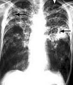
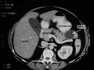
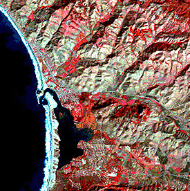
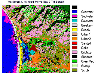

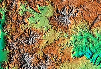
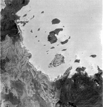
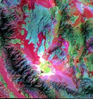
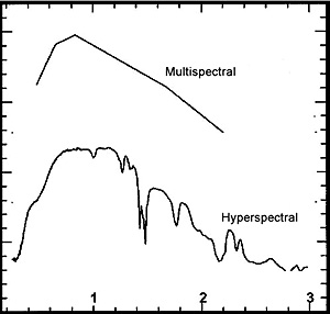

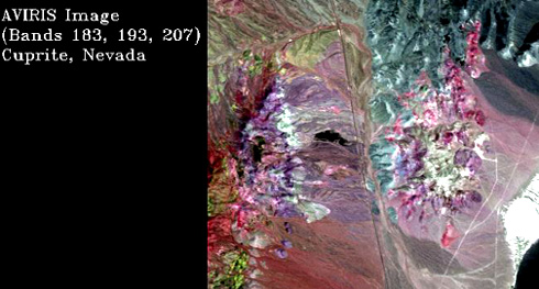

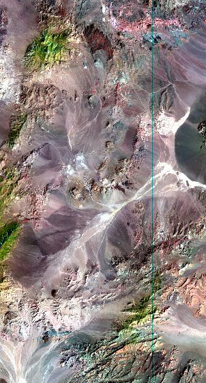
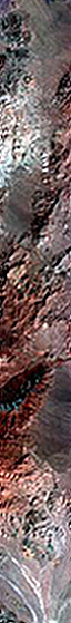


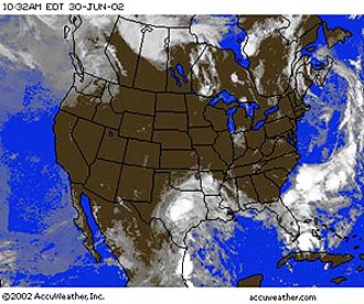
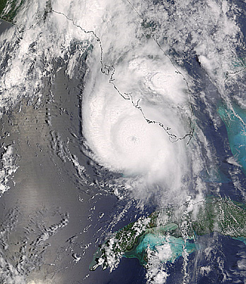
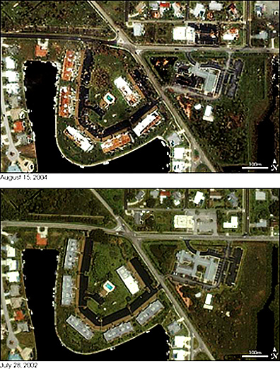
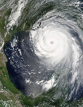
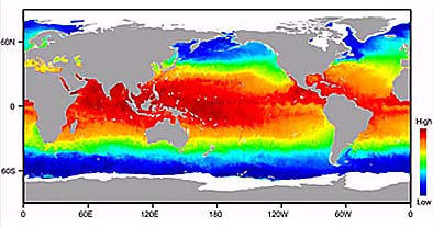
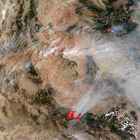
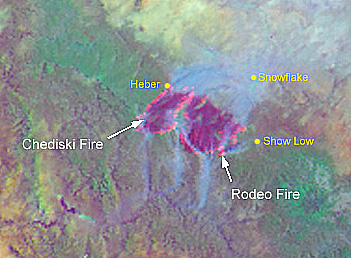
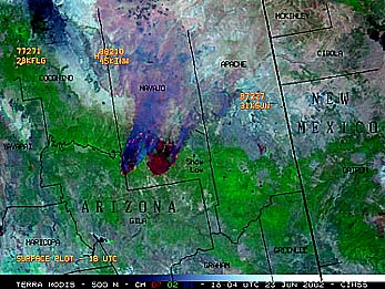
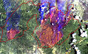

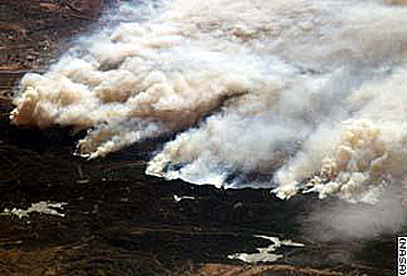
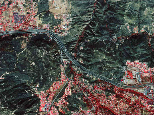
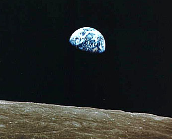

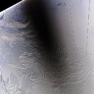
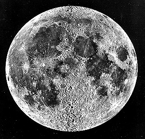
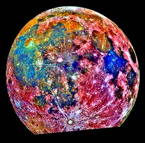
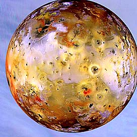
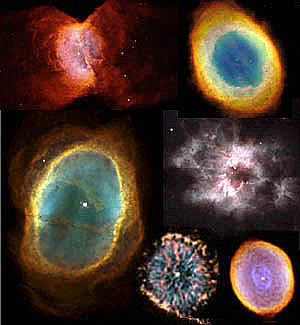
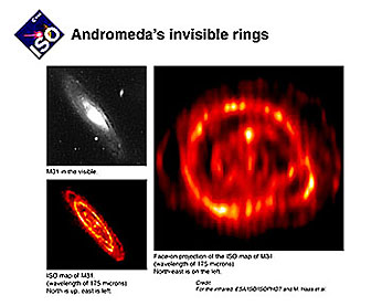

Collaborators: Code 935 NASA GSFC, GST, USAF
Academy