- Introduction
- 1. Introduction to Quantitative Analysis
- 2. Descriptive Statistics
- 3. T-test for Difference in Means and Hypothesis Testing
- 4. Bivariate linear regression models
- 5. Multiple linear regression models
- 6. Assumptions and Violations of Assumptions
- 7. Interactions
- 8. Panel Data, Time-Series Cross-Section Models
- 9. Binary models: Logit
- 10. Frequently Asked Questions
- 11. Optional Material
- 12. Datasets
- 13. R Resources
- 14. References
- Published with GitBook
4. Bivariate linear regression models
4.1 Seminar
Setting a Working Directory
Before you begin, make sure to set your working directory to a folder where your course related files such as R scripts and datasets are kept. We recommend that you create a PUBLG100 folder for all your work. Create this folder on N: drive if you're using a UCL computer or somewhere on your local disk if you're using a personal laptop.
Once the folder is created, use the setwd() function in R to set your working directory.
| Recommended Folder Location | R Function | |
|---|---|---|
| UCL Computers | N: Drive | setwd("N:/PUBLG100") |
| Personal Laptop (Windows) | C: Drive | setwd("C:/PUBLG100") |
| Personal Laptop (Mac) | Home Folder | setwd("~/PUBLG100") |
After you've set the working directory, verify it by calling the getwd() function.
getwd()
Now download the R script for this seminar from the "Download .R Script" button above, and save it to your PUBLG100 folder.
Required Packages
We're introducing two new packages in this week's seminar. The Zelig package provides functionality that simplifies some regression tasks, while texreg makes it easy to produce publication quality output from our regression models. We'll discuss these packages in more detail as we go along but for now let's just install them with the install.packages() function.
install.packages("Zelig")
install.packages("texreg")
Now, let's load Zelig, textreg and the dplyr package that we used last week. If you don't have dplyr installed for some reason then make sure to install it before loading.
NOTE: Make sure to load the packages in the order listed below. If you load Zelig after dplyr, then you might have to restart RStudio for your scripts to work properly.
library(texreg)
library(Zelig)
library(dplyr)
Clear the environment and set the working directory.
# clear environment
rm(list = ls())

# set working directory
# setwd(...)
Merging Datasets
Up until this point, we've been using datasets where all the variables of interest were available to us in a single file. Often times however, the variables we're interested in are not available from a single source and must be merged together to create a single dataset.
The dataset we're working with today is the California Test Score Data we've already seen in lectures and assigned text. The dataset is split into the following files:
| File | Description |
|---|---|
CASchoolAdmin.csv |
Administrative data for each school district, including number of enrolled students, number of teachers, average district income, etc. |
CAStudents.csv |
Student level data including reading and mathematics scores for each school. |
CABenefits.csv |
Benefits data including the percentage qualifying for CalWorks (income assistance) and reduced-price lunch for each school district. |
Download the first two datasets from the links below:
Download 'CASchoolAdmin' Dataset Download 'CAStudents' Dataset
Let's load the CASchoolAdmin.csv and CAStudents.csv datasets into R using read.csv() and find out if there are any variables that are common to both.
# load the California test score datasets
CA_admin <- read.csv("CASchoolAdmin.csv")
CA_students <- read.csv("CAStudents.csv")
Now let's see what the dataset looks like. We normally use the names() function to see what the variables are called, but we would also like to know what type of data is stored in each variable. We can use the str() function that gives us a bit more information about a dataset than the names() function.
names(CA_admin)
 [1] "district"    "school"      "county"      "grades"      "students"
 [6] "teachers"    "computer"    "expenditure" "income"      "english"
str(CA_admin)
'data.frame':   420 obs. of  10 variables:
 $ district   : int  75119 61499 61549 61457 61523 62042 68536 63834 62331 67306 ...
 $ school     : Factor w/ 409 levels "Ackerman Elementary",..: 362 214 367 134 270 53 152 383 263 93 ...
 $ county     : Factor w/ 45 levels "Alameda","Butte",..: 1 2 2 2 2 6 29 11 6 25 ...
 $ grades     : Factor w/ 2 levels "KK-06","KK-08": 2 2 2 2 2 2 2 2 2 1 ...
 $ students   : int  195 240 1550 243 1335 137 195 888 379 2247 ...
 $ teachers   : num  10.9 11.1 82.9 14 71.5 ...
 $ computer   : int  67 101 169 85 171 25 28 66 35 0 ...
 $ expenditure: num  6385 5099 5502 7102 5236 ...
 $ income     : num  22.69 9.82 8.98 8.98 9.08 ...
 $ english    : num  0 4.58 30 0 13.86 ...
Notice how read.csv() automatically converted both county and school to factor variables when loading the dataset.
Now, let's do the same for the students dataset.
names(CA_students)
[1] "county" "school" "read" "math"
str(CA_students)
'data.frame':   420 obs. of  4 variables:
 $ county: Factor w/ 45 levels "Alameda","Butte",..: 1 2 2 2 2 6 29 11 6 25 ...
 $ school: Factor w/ 409 levels "Ackerman Elementary",..: 362 214 367 134 270 53 152 383 263 93 ...
 $ read  : num  692 660 636 652 642 ...
 $ math  : num  690 662 651 644 640 ...
It seems that county and school are common to both datasets so we can use them to do the merge.
Now let's use the merge() function to merge these two datasets together. There are three arguments that we need to provide to the merge() function so it knows what we are trying to merge and how.
merge(x, y, by)
| Argument | Description |
|---|---|
x |
The first dataset to merge. This is the CA_admin dataset in our case. |
y |
The second dataset to merge. This is the CA_students dataset. |
by |
Name of the column or columns that are common in both datasets. We know that county and school are common to both datasets so we'll pass them as a vector by combining the two names together. |
For more information on how the merge() function works, type help(merge) in R.
# merge the two datasets
CA_schools <- merge(CA_admin, CA_students, by = c("county", "school"))

# explore dataset
names(CA_schools)
 [1] "county"      "school"      "district"    "grades"      "students"
 [6] "teachers"    "computer"    "expenditure" "income"      "english"
[11] "read"        "math"
head(CA_schools)
Dplyr mutate()
The mutate() function is used for adding new variables, or modifying existing ones in a dataframe. We saw an example of creating a new variable using the apply() function a couple of weeks ago, but now let's do something very similar with the mutate() function instead.
Our dataset includes the number of enrolled students and number of teachers for each district so we can easily use them to calculate a student-teacher ratio. We will call this new variable STR and calculate it by simply dividing the students variable by the teachers variable. We also would like to create a combined score from the average math and read scores for each school district. Again, calculating that is rather trivial as we just need to add the math and read scores and divide the result by 2.
We can create the student-teacher ratio (STR) and the score in one shot using the mutate() function.
CA_schools <- mutate(CA_schools,
                     STR = students / teachers,
                     score = (math + read) / 2)
Now that we've created the STR and score variables, let's visualize the data using a scatter plot.
Is there a correlation between Student-Teacher ratio and test scores?
plot(score ~ STR, data = CA_schools,
     xlab = "Student-Teacher Ratio",
     ylab = "Test Score")

In order to answer that question empirically, we will run linear regression using the lm() function in R. The lm() function needs to know the relationship we're trying to model and the dataset for our observations. The two arguments we need to provide to the lm() function are described below.
| Argument | Description |
|---|---|
formula |
The formula describes the relationship between the dependent and independent variables, for example dependent.variable ~ independent.variable. Recall from last week that we used something very similar with t-test when comparing the difference of means.In our case, we'd like to model the relationship using the formula: score ~ STR |
data |
This is simply the name of the dataset that contains the variable of interest. In our case, this is the merged dataset called CA_schools. |
For more information on how the lm() function works, type help(lm) or ?lm at the console in RStudio.
STR_model <- lm(score ~ STR, data = CA_schools)
The lm() function has modeled the relationship between score and STR and we've saved it in an object called STR_model. Let's use the summary() function to see what this linear model looks like.
summary(STR_model)
Call:
lm(formula = score ~ STR, data = CA_schools)

Residuals:
    Min      1Q  Median      3Q     Max
-47.727 -14.251   0.483  12.822  48.540

Coefficients:
            Estimate Std. Error t value Pr(>|t|)
(Intercept) 698.9329     9.4675  73.825  < 2e-16 ***
STR          -2.2798     0.4798  -4.751 2.78e-06 ***
---
Signif. codes:  0 '***' 0.001 '**' 0.01 '*' 0.05 '.' 0.1 ' ' 1

Residual standard error: 18.58 on 418 degrees of freedom
Multiple R-squared:  0.05124,   Adjusted R-squared:  0.04897
F-statistic: 22.58 on 1 and 418 DF,  p-value: 2.783e-06
Interpreting Regression Output
The output from lm() might seem overwhelming at first so let's break it down one item at a time.
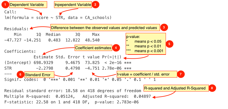
| # | Description |
|---|---|
 |
The dependent variable, also sometimes called the outcome variable. We are trying to model the effects of STR on score so score is the dependent variable. |
 |
The independent variable or the predictor variable. In our example, STR is the independent variable. |
 |
The differences between the observed values and the predicted values are called residuals. |
 |
The coefficients for the intercept and the independent variables. Using the coefficients we can write down the relationship between the dependent and the independent variables as: score = 698.9329493 + ( -2.2798081 * STR ) This tells us that for each unit increase in the variable STR, the score increases by -2.2798081. |
 |
The p-value of the model. Recall that according to the null hypotheses, the coefficient of interest is zero. The p-value tells us whether can can reject the null hypotheses or not. |
 |
The standard error estimates the standard deviation of the coefficients in our model. We can think of the standard error as the measure of precision for the estimated coefficients. |
 |
The t statistic is obtained by dividing the coefficients by the standard error. |
 |
The R-squared and adjusted R-squared tell us how much of the variance in our model is accounted for by the independent variable. The adjusted R-squared is always smaller than R-squared as it takes into account the number of independent variables and degrees of freedom. |
Now let's add a regression line to the scatter plot using the abline() function.
plot(score ~ STR, data = CA_schools,
     xlab = "Student-Teacher Ratio",
     ylab = "Test Score")
abline(STR_model, col = "red")

While the summary() function provides a slew of information about a fitted regression model, we often need to present our findings in easy to read tables similar to what you see in journal publications. The texreg package we installed earlier allows us to do just that.
Let's take a look at how to display the output of a regression model on the screen using the screenreg() function from texreg.
screenreg(STR_model)
=======================
             Model 1
-----------------------
(Intercept)  698.93 ***
              (9.47)
STR           -2.28 ***
              (0.48)
-----------------------
R^2            0.05
Adj. R^2       0.05
Num. obs.    420
RMSE          18.58
=======================
*** p < 0.001, ** p < 0.01, * p < 0.05
Returning to our example, are there other variables that might affect test scores in our dataset? For example, are test scores higher in school districts with higher levels of income?
Let's fit a linear model using income as the independent variable to answer that question.
income_model <- lm(score ~ income, data = CA_schools)
summary(income_model)
Call:
lm(formula = score ~ income, data = CA_schools)

Residuals:
    Min      1Q  Median      3Q     Max
-39.574  -8.803   0.603   9.032  32.530

Coefficients:
            Estimate Std. Error t value Pr(>|t|)
(Intercept) 625.3836     1.5324  408.11   <2e-16 ***
income        1.8785     0.0905   20.76   <2e-16 ***
---
Signif. codes:  0 '***' 0.001 '**' 0.01 '*' 0.05 '.' 0.1 ' ' 1

Residual standard error: 13.39 on 418 degrees of freedom
Multiple R-squared:  0.5076,    Adjusted R-squared:  0.5064
F-statistic: 430.8 on 1 and 418 DF,  p-value: < 2.2e-16
We can show regression line from the income_model just like we did with our first model.
plot(score ~ income, data = CA_schools,
     xlab = "District Income",
     ylab = "Test Score")
abline(income_model, col = "blue")

Does income_level offer a better fit than STR_model? Maybe we can answer that question by looking at the regression tables instead. Let's print the two models side-by-side in a single table with screenreg().
screenreg(list(STR_model, income_model))
===================================
             Model 1     Model 2
-----------------------------------
(Intercept)  698.93 ***  625.38 ***
              (9.47)      (1.53)
STR           -2.28 ***
              (0.48)
income                     1.88 ***
                          (0.09)
-----------------------------------
R^2            0.05        0.51
Adj. R^2       0.05        0.51
Num. obs.    420         420
RMSE          18.58       13.39
===================================
*** p < 0.001, ** p < 0.01, * p < 0.05
Finally, let's save the same output as a Microsoft Word document using htmlreg().
htmlreg(list(STR_model, income_model), file = "California_Schools.doc")
The table was written to the file 'California_Schools.doc'.
Predictions and Confidence Interval
We will use the Zelig package since it provides convenient functions for making predictions and plotting confidence intervals. First, let's go back to our last model where we used income as the independent variable but this time estimate the model using the Zelig package. The arguments for the zelig() function are very similar to what we used with lm(). The only difference is that we need to tell Zelig what type of model we're trying to estimate.
| Argument | Description |
|---|---|
formula |
The formula is the describes the relationship between the dependent and independent variables, for example dependent.variable ~ independent.variable. |
data |
This is the name of the dataset that contains the variable of interest. |
model |
This is where we tell Zelig the type of model to estimate. Since we're interested in a Least Squares regression model, we will use model = "ls" argument. |
z.out <- zelig(score ~ income, data = CA_schools, model = "ls")
How to cite this model in Zelig:
  R Core Team. 2007.
  ls: Least Squares Regression for Continuous Dependent Variables
  in Christine Choirat, James Honaker, Kosuke Imai, Gary King, and Olivia Lau,
  "Zelig: Everyone's Statistical Software," http://zeligproject.org/
We've saved the model estimated with zelig() in an object called z.out. We can call it anything we want, but Zelig documentation generally uses z.out so we'll do the same. We can use the summary() function exactly the same way as we used it with lm() to print out the estimated model.
summary(z.out)
Model:

Call:
z5$zelig(formula = score ~ income, data = CA_schools)

Residuals:
    Min      1Q  Median      3Q     Max
-39.574  -8.803   0.603   9.032  32.530

Coefficients:
            Estimate Std. Error t value Pr(>|t|)
(Intercept) 625.3836     1.5324  408.11   <2e-16
income        1.8785     0.0905   20.76   <2e-16

Residual standard error: 13.39 on 418 degrees of freedom
Multiple R-squared:  0.5076,    Adjusted R-squared:  0.5064
F-statistic: 430.8 on 1 and 418 DF,  p-value: < 2.2e-16

Next step: Use 'setx' method
Next, let's use Zelig's setx() and sim() functions for making predictions and plotting confidence intervals.
x.out <- setx(z.out, income = seq(min(CA_schools$income), max(CA_schools$income), 1))
s.out <- sim(z.out, x = x.out)
Again, we're following Zelig convention of using x.out and s.out as the names of the objects created from setx() and sim().
Now let's take a look at the summary of the simulations run by Zelig.
NOTE: We've truncated the output to only include a small subset of the output generated by summary.
summary(s.out)
[1] 5.335


 sim range :
 -----
ev
      mean       sd      50%    2.5%    97.5%
1 635.4546 1.142503 635.3945 633.241 637.6818
pv
         mean      sd      50%     2.5%    97.5%
[1,] 635.5079 13.8709 635.0691 608.2508 662.6071


[1] 6.335


 sim range :
 -----
ev
      mean       sd      50%     2.5%    97.5%
1 637.3264 1.071294 637.2691 635.2157 639.3698
pv
         mean       sd     50%    2.5%    97.5%
[1,] 636.5395 13.85414 636.399 609.564 662.7647


[1] 7.335


 sim range :
 -----
ev
      mean       sd     50%     2.5%    97.5%
1 639.1982 1.003129 639.143 637.1811 641.1293
pv
         mean       sd      50%     2.5%    97.5%
[1,] 638.9055 13.63499 638.4329 613.4762 665.5108


....
Finally, we can plot the confidence interval using the ci.plot function.
ci.plot(s.out, ci = 95, xlab = "District Income (in USD $1000)")

Additional Resources
Linear Regression Interactive App
Exercises
Download the
CABenefits.csvfrom the link below and merge it with theCAStudents.csvdataset.- Download 'CABenefits' Dataset
- HINT: Pay close attention to the variables in ALL 3 datasets including
CASchoolAdmin.csv. Just looking atCABenefits.csvandCAStudents.csvwouldn't be enough since they don't have any common variables.
Estimate a model explaining the relationship between test scores and the percentage qualifying for CalWorks income assistance?
- Plot the regression line of the model.
- How does this model compare to the models we estimated in the seminar with
STRandincomeas independent variables? Present your findings by comparing the output of all three models in side-by-side tables using thetexregpackage. - Save your model comparison table to a Microsoft Word document (or another format if you don't use Word).
- Generate predicted values from the fitted model with
calworksand plot the confidence interval using Zelig. - Save all the plots as graphics files.
- Hint: Look at the Plot window in RStudio for an option to save your plot. Alternatively, you can use the
png()function for saving the graphics file directly from your R script.
- Hint: Look at the Plot window in RStudio for an option to save your plot. Alternatively, you can use the